Mathematical preliminaries
Preliminary note 1 of 2 · Jhony H. Giraldo · Télécom Paris, Institut Polytechnique de Paris
This note covers the linear algebra the six lectures actually use — and deliberately nothing more. It is not a linear algebra course. Every section ends with Where this is used, naming the lecture and the equation that needs it, so you can read it front to back now or return to a single section when a lecture stops making sense.
There are no proofs of the big theorems here. There are worked numbers, because a matrix identity you have evaluated once on a four-node graph is worth more than one you have only read.
1 Diagnostic: what do you actually need to read?
Ten questions. Each names the section that covers it. If you can answer one comfortably, skip that section.
- For \(\mathbf{A}\in\mathbb{R}^{4\times4}\) and \(\mathbf{x}\in\mathbb{R}^{4}\), what does entry \(i\) of \(\mathbf{A}\mathbf{x}\) equal as a sum? (Products)
- If \(\mathbf{A}\) is a graph's adjacency matrix, what does \((\mathbf{A}^2)_{ij}\) count? (Products)
- What does \(\mathbf{P}\mathbf{A}\mathbf{P}^{\top}\) do, for \(\mathbf{P}\) a permutation matrix? (Structured matrices)
- A graph has \(N=10^{6}\) nodes and \(10^{7}\) edges. How much memory does its adjacency matrix need, dense and sparse? (Structured matrices)
- State what the spectral theorem guarantees for a real symmetric matrix. (Eigenvalues)
- \(\mathbf{S}\) is symmetric with eigenvalues in \((-1,1]\). Describe \(\mathbf{S}^{k}\mathbf{x}\) as \(k\to\infty\). (Matrix powers)
- What is \(\mathbf{x}^{\top}\mathbf{L}\mathbf{x}\) when \(\mathbf{L}\) is a graph Laplacian, written as a sum over edges? (Eigenvalues)
- Differentiate \(f(\mathbf{x})=\mathbf{x}^{\top}\mathbf{A}\mathbf{x}\) with respect to \(\mathbf{x}\), for symmetric \(\mathbf{A}\). (Matrix calculus)
- What is \(\nabla_{\mathbf{Z}}\operatorname{tr}(\mathbf{Z}^{\top}\mathbf{A}\mathbf{Z})\)? (Matrix calculus)
- If \(\mathbf{U}\in\mathbb{R}^{N\times d}\) and \(\mathbf{V}\in\mathbb{R}^{M\times d}\) with \(d\ll N,M\), what is the maximum rank of \(\mathbf{U}\mathbf{V}^{\top}\), and why does that matter? (Rank)
- \((\mathbf{A}\mathbf{x})_i=\sum_{j=1}^{4}A_{ij}x_j\) — a weighted sum of the entries of \(\mathbf{x}\) at \(i\)'s neighbours.
- The number of walks of length \(2\) from \(i\) to \(j\); on the diagonal, \((\mathbf{A}^2)_{ii}=\deg(i)\). Unweighted graphs only.
- It relabels the nodes: \((\mathbf{P}\mathbf{A}\mathbf{P}^{\top})\) is the adjacency matrix of the same graph under the permutation \(\mathbf{P}\) encodes. The graph is unchanged, only its indexing is.
- Dense: \(N^2=10^{12}\) entries, about \(4\) TB at 4 bytes each. Sparse (CSR): \(\mathcal{O}(|\mathcal{E}|)\), a few hundred MB. This gap is why every method in the course is written in terms of sparse products.
- A real symmetric \(\mathbf{A}\) has an orthonormal basis of eigenvectors with real eigenvalues: \(\mathbf{A}=\mathbf{U}\boldsymbol{\Lambda}\mathbf{U}^{\top}\), \(\mathbf{U}^{\top}\mathbf{U}=\mathbf{I}\).
- Components along eigenvectors with \(|\lambda|<1\) decay geometrically, so \(\mathbf{S}^{k}\mathbf{x}\) converges to its projection onto the \(\lambda=1\) eigenspace. If that eigenspace is one-dimensional and spanned by a unit \(\mathbf{u}\), the limit is \((\mathbf{u}^{\top}\mathbf{x})\,\mathbf{u}\).
- \(\mathbf{x}^{\top}\mathbf{L}\mathbf{x}=\sum_{(i,j)\in\mathcal{E}}(x_i-x_j)^2\) — the total squared variation across edges, and the reason \(\mathbf{L}\) measures smoothness.
- \(\nabla_{\mathbf{x}}f=2\mathbf{A}\mathbf{x}\) when \(\mathbf{A}\) is symmetric (in general \((\mathbf{A}+\mathbf{A}^{\top})\mathbf{x}\)).
- \(\nabla_{\mathbf{Z}}\operatorname{tr}(\mathbf{Z}^{\top}\mathbf{A}\mathbf{Z})=(\mathbf{A}+\mathbf{A}^{\top})\mathbf{Z}\), which is \(2\mathbf{A}\mathbf{Z}\) for symmetric \(\mathbf{A}\).
- At most \(d\). It matters because a rank-\(d\) factorization stores \(d(N+M)\) numbers instead of \(NM\), and cannot represent an interaction pattern of higher rank — the modelling assumption behind every embedding method in Lecture 5.
2 The running example
Everything below is illustrated on one graph, so that each new object lands on something familiar.
It is a small four-node graph of its own. Lecture 1 uses a similar one for its adjacency-matrix example, but that graph carries an extra edge \(\{3,4\}\) and so has degrees \([2,3,2,3]\); this one omits it, giving degrees \([2,3,1,2]\). The asymmetry is deliberate — a node of degree \(1\) makes degree normalization visible in a way a regular graph would hide.
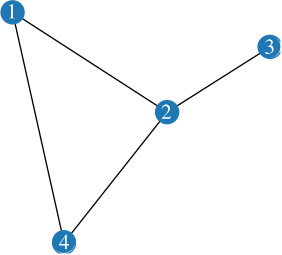
Its adjacency matrix, degree matrix and Laplacian are
\[ \mathbf{A}= \begin{bmatrix} 0&1&0&1\\ 1&0&1&1\\ 0&1&0&0\\ 1&1&0&0 \end{bmatrix}, \qquad \mathbf{D}= \begin{bmatrix} 2&&&\\&3&&\\&&1&\\&&&2 \end{bmatrix}, \qquad \mathbf{L}=\mathbf{D}-\mathbf{A}. \]
Read \(\mathbf{A}\) row by row: row 2 has ones in columns 1, 3 and 4, because node 2 is adjacent to those three. \(\mathbf{D}\) holds the row sums. Keep this matrix in view — it reappears in every section.
3 Vectors, matrices, and what a product means
3.1 The two readings of \(\mathbf{A}\mathbf{x}\)
For \(\mathbf{A}\in\mathbb{R}^{m\times n}\) and \(\mathbf{x}\in\mathbb{R}^{n}\), the product \(\mathbf{y}=\mathbf{A}\mathbf{x}\in\mathbb{R}^{m}\) has entries
\[ y_i=\sum_{j=1}^{n}A_{ij}x_j . \]
That is the definition. But there are two readings, and switching between them is most of what fluency in this subject means.
Row reading. \(y_i\) is the inner product of row \(i\) of \(\mathbf{A}\) with \(\mathbf{x}\). Each output is a weighted sum of the input.
Column reading. \(\mathbf{y}=\sum_{j}x_j\,\mathbf{a}_{:j}\), a weighted sum of the columns of \(\mathbf{A}\). The output lives in the span of the columns.
Worked example — \(\mathbf{A}\mathbf{x}\) is one round of message passing
Take \(\mathbf{x}=[1,0,0,0]^{\top}\): a value of one at node 1, zero elsewhere. Then
\[ \mathbf{A}\mathbf{x}= \begin{bmatrix} 0&1&0&1\\1&0&1&1\\0&1&0&0\\1&1&0&0 \end{bmatrix} \begin{bmatrix}1\\0\\0\\0\end{bmatrix} =\begin{bmatrix}0\\1\\0\\1\end{bmatrix}. \]
The column reading makes this immediate: we picked out column 1 of \(\mathbf{A}\), which is exactly the indicator of node 1’s neighbors.
This is the single most important fact in the course. Multiplying a signal by the adjacency matrix moves each node’s value to its neighbors. Every graph neural network in Lectures 2 to 6 is built from this operation.
Now take a general \(\mathbf{x}\). Row \(i\) gives \(y_i=\sum_{j}A_{ij}x_j=\sum_{j\in\mathcal{N}_i}x_j\): each node receives the sum of its neighbors’ values.
3.2 Matrix–matrix products, and walks
For \(\mathbf{A}\in\mathbb{R}^{m\times n}\) and \(\mathbf{B}\in\mathbb{R}^{n\times p}\),
\[ (\mathbf{A}\mathbf{B})_{ij}=\sum_{k=1}^{n}A_{ik}B_{kj}, \]
which is \(\mathbf{A}\) applied to each column of \(\mathbf{B}\) — composition of the two linear maps. The inner dimensions must match, and the result is \(m\times p\). Checking shapes before anything else will save you more debugging time than any other habit; Lecture 2 has a worked example that does nothing but track shapes through a two-layer network.
Matrix multiplication is associative (\((\mathbf{A}\mathbf{B})\mathbf{C}=\mathbf{A}(\mathbf{B}\mathbf{C})\)) but not commutative (\(\mathbf{A}\mathbf{B}\neq\mathbf{B}\mathbf{A}\) in general). Associativity is not a formality — it is what lets Lecture 3 collapse a stack of weight matrices into one.
Worked example — \(\mathbf{A}^2\) counts length-two walks
\[ \mathbf{A}^2= \begin{bmatrix} 2&1&1&1\\ 1&3&0&1\\ 1&0&1&1\\ 1&1&1&2 \end{bmatrix}. \]
Why? By definition \((\mathbf{A}^2)_{ij}=\sum_k A_{ik}A_{kj}\), and the term \(A_{ik}A_{kj}\) is \(1\) exactly when \(i\!-\!k\) and \(k\!-\!j\) are both edges — that is, when \(k\) is the middle of a two-step walk from \(i\) to \(j\). So the sum counts length-two walks from \(i\) to \(j\).
Check the diagonal: \((\mathbf{A}^2)_{22}=3\), because from node 2 you can step out to any of its three neighbors and come straight back. In general \((\mathbf{A}^2)_{ii}=d_i\).
Check an off-diagonal: \((\mathbf{A}^2)_{13}=1\), the single walk \(1\to2\to3\). And \((\mathbf{A}^2)_{23}=0\) — there is no two-step walk from 2 to 3, even though they are adjacent, because a one-step edge is not a two-step walk.
The general statement is that for an unweighted adjacency matrix, \((\mathbf{A}^{k})_{ij}\) counts walks of length exactly \(k\). On a weighted graph the same sum still runs over walks, but each contributes the product of its edge weights rather than \(1\), so the entry is a weighted walk total rather than a count. Either way, powers of \(\mathbf{A}\) describe reach on a graph, and this is the seed of the diffusion sequence in Lecture 2.
3.3 Inner products, norms, orthogonality
For \(\mathbf{u},\mathbf{v}\in\mathbb{R}^{n}\),
\[ \langle\mathbf{u},\mathbf{v}\rangle=\mathbf{u}^{\top}\mathbf{v}=\sum_{i}u_iv_i, \qquad \|\mathbf{u}\|_2=\sqrt{\mathbf{u}^{\top}\mathbf{u}}, \qquad \mathbf{u}^{\top}\mathbf{v}=\|\mathbf{u}\|\,\|\mathbf{v}\|\cos\theta . \]
Two vectors are orthogonal when \(\mathbf{u}^{\top}\mathbf{v}=0\), and orthonormal when additionally each has unit norm.
The inner product is how similarity gets measured throughout the course: it is the score \(\mathbf{z}_u^{\top}\mathbf{z}_v\) between a user and an item in Lecture 5, and the decoder between two node embeddings in Lecture 1. Note what it conflates — a large \(\mathbf{u}^{\top}\mathbf{v}\) can mean the vectors point the same way or simply that one is long. When only direction should matter, normalize first.
3.4 Transpose
\((\mathbf{A}^{\top})_{ij}=A_{ji}\), and \((\mathbf{A}\mathbf{B})^{\top}=\mathbf{B}^{\top}\mathbf{A}^{\top}\) — the order reverses. A matrix is symmetric when \(\mathbf{A}=\mathbf{A}^{\top}\).
For a graph this is not a technical detail: an undirected graph always has a symmetric adjacency matrix. The converse needs care — a directed graph in which every edge is reciprocated also has a symmetric \(\mathbf{A}\), and is indistinguishable from the undirected one at the level of the matrix. What matters downstream is the symmetry, since that is what the spectral guarantees below require. Lecture 1’s directed example has \(A_{13}=1\) but \(A_{31}=0\), so it is genuinely asymmetric.
Where this is used
\(\mathbf{A}\mathbf{x}\) as message passing is Lecture 2’s diffusion section and every model after it. \((\mathbf{A}^{2})_{ij}\) as a walk count is Lecture 1’s worked example and Exercise 1. Inner-product scoring is Lecture 1’s decoder and Lecture 5’s \(\operatorname{score}(u,v)=\langle\mathbf{u},\mathbf{v}\rangle\). Shape tracking is Lecture 2’s two-layer GCN example.
4 Structured and sparse matrices
Most matrices in this course are not arbitrary. Recognizing the structure is what makes them cheap.
4.1 Diagonal matrices
\(\mathbf{D}=\operatorname{diag}(d_1,\dots,d_N)\) has entries only on the diagonal. Then \(\mathbf{D}\mathbf{x}\) scales entry \(i\) by \(d_i\), \(\mathbf{D}\mathbf{A}\) scales row \(i\) of \(\mathbf{A}\) by \(d_i\), and \(\mathbf{A}\mathbf{D}\) scales column \(j\) by \(d_j\). Inversion is entrywise: \(\mathbf{D}^{-1}=\operatorname{diag}(1/d_i)\), and likewise \(\mathbf{D}^{-1/2}=\operatorname{diag}(1/\sqrt{d_i})\).
That last one is worth pausing on, because it appears in nearly every equation from Lecture 2 onward:
\[ \left(\mathbf{D}^{-1/2}\mathbf{A}\mathbf{D}^{-1/2}\right)_{ij}=\frac{A_{ij}}{\sqrt{d_i d_j}} . \]
Left-multiplying scales rows, right-multiplying scales columns, so the entry picks up both factors. This is the symmetric normalization, and knowing it is a two-sided scaling explains a property that catches people out: it is not generally row-stochastic. Its rows sum to one only when the graph is regular, where \(\sqrt{d_id_j}=d\) for every edge and the two-sided scaling collapses to a one-sided one. On an irregular graph the rows do not sum to one, and they do not even sum to the same value. (The operator that is always row-stochastic is \(\mathbf{D}^{-1}\mathbf{A}\), the random-walk matrix.)
Worked example — symmetric normalization on the running graph
With \(\mathbf{d}=[2,3,1,2]\),
\[ \hat{\mathbf{A}}=\mathbf{D}^{-1/2}\mathbf{A}\mathbf{D}^{-1/2}= \begin{bmatrix} 0 & \tfrac{1}{\sqrt{6}} & 0 & \tfrac{1}{2}\\[3pt] \tfrac{1}{\sqrt{6}} & 0 & \tfrac{1}{\sqrt{3}} & \tfrac{1}{\sqrt{6}}\\[3pt] 0 & \tfrac{1}{\sqrt{3}} & 0 & 0\\[3pt] \tfrac{1}{2} & \tfrac{1}{\sqrt{6}} & 0 & 0 \end{bmatrix} \approx \begin{bmatrix} 0&0.408&0&0.5\\ 0.408&0&0.577&0.408\\ 0&0.577&0&0\\ 0.5&0.408&0&0 \end{bmatrix}. \]
Row 1 sums to \(0.908\), row 2 to \(1.393\). Not one, and not even constant across rows. Note also that the high-degree node 2 receives smaller coefficients from its neighbors — degree normalization damps hubs, which is the mechanism behind Lecture 2’s GCN-versus-GAT comparison.
4.2 Permutation matrices
A permutation matrix \(\mathbf{P}\) has exactly one \(1\) in each row and column, zeros elsewhere. It is orthogonal: \(\mathbf{P}^{\top}\mathbf{P}=\mathbf{I}\), so \(\mathbf{P}^{-1}=\mathbf{P}^{\top}\).
\(\mathbf{P}\mathbf{x}\) reorders the entries of \(\mathbf{x}\). \(\mathbf{P}\mathbf{A}\) reorders the rows of \(\mathbf{A}\); \(\mathbf{A}\mathbf{P}^{\top}\) reorders the columns. So
\[ \mathbf{A}'=\mathbf{P}\mathbf{A}\mathbf{P}^{\top} \]
reorders rows and columns consistently — it is the same graph with its nodes relabelled.
Why this matters more than it looks
A graph has no canonical node ordering. The labels \(1,2,3,4\) were our choice, and any other choice describes the same object. So a model of a graph should not depend on them.
Two properties formalize this. A node-level map \(f\) is permutation equivariant if
\[ f(\mathbf{P}\mathbf{A}\mathbf{P}^{\top},\mathbf{P}\mathbf{X})=\mathbf{P}f(\mathbf{A},\mathbf{X}) \]
— relabel the input, and the output is relabelled the same way. A graph-level map \(g\) is permutation invariant if \(g(\mathbf{P}\mathbf{A}\mathbf{P}^{\top},\mathbf{P}\mathbf{X})=g(\mathbf{A},\mathbf{X})\) — the output does not change at all.
One identity does most of the work: since \(\mathbf{P}^{\top}\mathbf{P}=\mathbf{I}\),
\[ (\mathbf{P}\mathbf{A}\mathbf{P}^{\top})^{k} =\mathbf{P}\mathbf{A}\underbrace{\mathbf{P}^{\top}\mathbf{P}}_{\mathbf{I}}\mathbf{A}\mathbf{P}^{\top}\cdots =\mathbf{P}\mathbf{A}^{k}\mathbf{P}^{\top}, \]
so every polynomial in the adjacency matrix is automatically equivariant. That single line is why Lecture 2 can define graph convolution as a polynomial in a shift operator and get the right invariance for free.
4.3 Sparsity
A matrix is sparse when almost all entries are zero. Real graphs are extremely sparse: a social network with \(N=10^{6}\) users and \(100\) friends each has \(10^{8}\) nonzeros out of \(10^{12}\) entries — one in ten thousand.
Storage format, not mathematics, is what changes:
| format | stores | memory |
|---|---|---|
| dense array | every entry | \(O(N^{2})\) |
coordinate / edge_index |
one \((i,j)\) pair per stored edge, plus a value if weighted | \(O(|\mathcal{E}|)\) |
| compressed sparse row | values, column indices, row offsets | \(O(N+|\mathcal{E}|)\) |
Worked example — why dense storage fails
Take \(N=10^{6}\) nodes with \(100\) neighbors each, so \(|\mathcal{E}|=5\times10^{7}\) undirected edges, at 8 bytes per number.
Dense: \(8N^{2}=8\times10^{12}\) bytes \(=8\) terabytes.
Edge list: two indices per stored direction, \(8\times2\times2|\mathcal{E}|=1.6\times10^{9}\) bytes \(=1.6\) gigabytes.
A factor of five thousand, and the difference between impossible and routine. The same arithmetic at \(N=25\times10^{6}\) is Lecture 2’s worked example.
The cost of a product changes too. Dense \(\mathbf{A}\mathbf{x}\) costs \(O(N^{2})\) multiply–adds; sparse costs \(O(|\mathcal{E}|)\), since zero entries contribute nothing. This is the origin of the \(O(|\mathcal{E}|)\) complexity quoted throughout the course.
A trap worth knowing before Lecture 2
Sparsity is not preserved by powers. \(\mathbf{A}\) may be sparse while \(\mathbf{A}^{k}\) is dense — \((\mathbf{A}^{k})_{ij}\neq0\) whenever any length-\(k\) walk joins \(i\) to \(j\), and on a well-connected graph that is soon almost every pair.
The consequence is a rule you will meet repeatedly: to compute \(\mathbf{A}^{k}\mathbf{x}\), never form \(\mathbf{A}^{k}\). Iterate instead,
\[ \mathbf{x}\leftarrow\mathbf{A}\mathbf{x}\quad k\text{ times}, \]
which costs \(O(k|\mathcal{E}|)\) and never stores anything denser than \(\mathbf{A}\).
Where this is used
Symmetric normalization is the GCN operator of Lecture 2 and the LightGCN operator of Lecture 5. Permutation equivariance is Lecture 1’s section on why graph learning is different and the justification for graph convolution in Lecture 2. Sparse storage and the \(O(N^{2})\)-versus-\(O(N+|\mathcal{E}|)\) contrast are Lecture 1’s representation section and Lecture 3’s memory-wall example. The “never form \(\mathbf{S}^{k}\)” rule is Lecture 2’s Check 2.
5 Eigenvalues, eigenvectors, and quadratic forms
5.1 The definition, and what it buys
A nonzero \(\mathbf{u}\) is an eigenvector of \(\mathbf{A}\) with eigenvalue \(\lambda\) when
\[ \mathbf{A}\mathbf{u}=\lambda\mathbf{u}. \]
Along an eigenvector, the matrix does nothing but scale. If we can write a vector in terms of eigenvectors, we can apply the matrix by scaling each piece — and that turns matrix products into arithmetic on numbers.
5.2 The spectral theorem
The one theorem to remember
If \(\mathbf{A}\in\mathbb{R}^{N\times N}\) is symmetric, then:
- all its eigenvalues are real;
- it has an orthonormal basis of eigenvectors \(\mathbf{u}_1,\dots,\mathbf{u}_N\);
- it factors as \(\mathbf{A}=\mathbf{U}\boldsymbol{\Lambda}\mathbf{U}^{\top}\), with \(\mathbf{U}=[\mathbf{u}_1\cdots\mathbf{u}_N]\) orthogonal (\(\mathbf{U}^{\top}\mathbf{U}=\mathbf{U}\mathbf{U}^{\top}=\mathbf{I}\)) and \(\boldsymbol{\Lambda}=\operatorname{diag}(\lambda_1,\dots,\lambda_N)\).
We take this without proof. What matters is the licence it gives: for symmetric matrices, the eigenvectors form a coordinate system, and \(\mathbf{U}^{-1}=\mathbf{U}^{\top}\) makes moving in and out of it free.
Symmetry is a real condition, not boilerplate. A general square matrix may have complex eigenvalues, or too few eigenvectors to form a basis. This is why Lecture 4 fixes an undirected graph with a symmetric Laplacian before defining the graph Fourier transform: the whole construction rests on clause 2.
Writing \(\mathbf{x}=\sum_i c_i\mathbf{u}_i\) with \(c_i=\mathbf{u}_i^{\top}\mathbf{x}\),
\[ \mathbf{A}\mathbf{x}=\sum_i \lambda_i c_i\mathbf{u}_i . \]
The matrix scales each coordinate by its eigenvalue and does nothing else. Every spectral argument in this course is a consequence of that one line.
5.3 Quadratic forms and the Laplacian
For symmetric \(\mathbf{A}\), the quadratic form is the scalar \(\mathbf{x}^{\top}\mathbf{A}\mathbf{x}=\sum_{i,j}A_{ij}x_ix_j\). Classify \(\mathbf{A}\) by its sign:
- positive definite if \(\mathbf{x}^{\top}\mathbf{A}\mathbf{x}>0\) for all \(\mathbf{x}\neq\mathbf{0}\), equivalently all \(\lambda_i>0\);
- positive semi-definite (PSD) if \(\mathbf{x}^{\top}\mathbf{A}\mathbf{x}\geq0\), equivalently all \(\lambda_i\geq0\).
The graph Laplacian \(\mathbf{L}=\mathbf{D}-\mathbf{A}\) is the quadratic form that matters here, and it has a remarkable identity.
Worked example — the Laplacian quadratic form is a sum over edges
Expanding \(\mathbf{x}^{\top}\mathbf{L}\mathbf{x}=\mathbf{x}^{\top}\mathbf{D}\mathbf{x}-\mathbf{x}^{\top}\mathbf{A}\mathbf{x}=\sum_i d_ix_i^{2}-\sum_{i,j}A_{ij}x_ix_j\) and using \(d_i=\sum_j A_{ij}\),
\[ \mathbf{x}^{\top}\mathbf{L}\mathbf{x}=\sum_{(i,j)\in\mathcal{E}}A_{ij}(x_i-x_j)^{2}. \]
It measures how much the signal changes along edges — nothing else. Non-adjacent nodes contribute no direct term.
Two immediate consequences. \(\mathbf{L}\) is PSD, since every term is a square times a nonnegative weight. And \(\mathbf{x}^{\top}\mathbf{L}\mathbf{x}=0\) exactly when \(x_i=x_j\) across every edge — so the constant vector \(\mathbf{1}\) satisfies \(\mathbf{L}\mathbf{1}=\mathbf{0}\), and \(\lambda_1=0\) is always an eigenvalue.
On the running graph with \(\mathbf{x}=[1,1,1,1]^{\top}\): every difference is zero, so \(\mathbf{x}^{\top}\mathbf{L}\mathbf{x}=0\). With \(\mathbf{x}=[1,-1,1,-1]^{\top}\): edges \(\{1,2\}\), \(\{2,3\}\) and \(\{1,4\}\) each contribute \((2)^{2}=4\), edge \(\{2,4\}\) contributes \(0\), giving \(12\).
Because \(\lambda_1=0\) always, \(\mathbf{L}\) is PSD but never positive definite, and never invertible. Lecture 4 turns this into a problem and then fixes it by adding \(\epsilon\mathbf{I}\).
5.4 The Rayleigh quotient
The quadratic form has no maximum on its own — scaling \(\mathbf{x}\) by \(c\) scales it by \(c^{2}\). Normalizing gives the Rayleigh quotient
\[ R(\mathbf{x})=\frac{\mathbf{x}^{\top}\mathbf{A}\mathbf{x}}{\mathbf{x}^{\top}\mathbf{x}}, \qquad \lambda_{\min}\leq R(\mathbf{x})\leq\lambda_{\max}, \]
with the bounds attained at the corresponding eigenvectors. It is the scale-free measure of “how much variation”, and the reason Lecture 4 has to distinguish a signal with small total variation from a signal that is smooth.
Where this is used
The spectral theorem underwrites the graph Fourier transform in Lecture 4’s spectral section. The Laplacian quadratic form is Lecture 4’s Definition 7 and its smoothness regularizer. PSD and definiteness return in Lecture 4’s Hessian analysis. The Rayleigh quotient is what Lecture 4’s Check 4 uses to separate amplitude from smoothness.
6 What matrix powers do
This section is short, and it is the most important one in the note. Over-smoothing in Lecture 2, low-pass filtering in Lecture 2 and 4, diffusion in Lecture 2, SGC in Lecture 3, LightGCN in Lecture 5 and power iteration in Lecture 1 are all the same fact.
Let \(\mathbf{S}\) be symmetric with eigendecomposition \(\mathbf{S}=\mathbf{U}\boldsymbol{\Lambda}\mathbf{U}^{\top}\). Then
\[ \mathbf{S}^{k}=\mathbf{U}\boldsymbol{\Lambda}^{k}\mathbf{U}^{\top}, \]
because the inner \(\mathbf{U}^{\top}\mathbf{U}=\mathbf{I}\) factors cancel. Writing \(\mathbf{x}=\sum_i c_i\mathbf{u}_i\),
\[ \mathbf{S}^{k}\mathbf{x}=\sum_{i}\lambda_i^{k}\,c_i\,\mathbf{u}_i . \]
Applying \(\mathbf{S}\) \(k\) times raises each eigenvalue to the \(k\)-th power and leaves the eigenvectors alone. Everything follows from reading off what \(\lambda^{k}\) does.
The four regimes
Sort by \(|\lambda_i|\) and let \(k\) grow.
| \(\lambda\) | \(\lambda^{k}\) as \(k\to\infty\) | what you see |
|---|---|---|
| \(\lambda=1\) | stays \(1\) | this component survives untouched |
| \(\vert\lambda\vert<1\) | \(\to0\) | this component is erased, geometrically fast |
| \(\lambda=-1\) | alternates \(-1,+1,\dots\) | survives in magnitude, flips sign every step |
| \(\vert\lambda\vert>1\) | \(\vert\lambda^{k}\vert\to\infty\) | blows up (alternating in sign if \(\lambda<-1\)) |
So repeated application is a filter: it keeps whatever lives at the extremes of the spectrum and destroys everything in the middle. Which components survive depends only on where their eigenvalues sit.
Three consequences you will meet by name:
Scope first: this is about a fixed linear operator
Everything in this section concerns applying one fixed matrix repeatedly, with no weights and no nonlinearity. A trained network interleaves \(\mathbf{W}^{(\ell)}\) and \(\sigma\), which are not diagonal in this eigenbasis, so the composition is not a spectral filter and needs its own analysis. Read what follows as the behaviour of the propagation, which is one ingredient of a GNN rather than the whole of it.
Over-smoothing (Lecture 2). Take the GCN operator \(\mathbf{S}=\tilde{\mathbf{D}}^{-1/2}\tilde{\mathbf{A}}\tilde{\mathbf{D}}^{-1/2}\) on a connected graph with self-loops. Its largest eigenvalue is \(1\), with unit eigenvector \(\mathbf{u}\propto\sqrt{\tilde{\mathbf{d}}}\), and every other eigenvalue satisfies \(|\lambda|<1\). So
\[ \mathbf{S}^{k}\mathbf{X}\;\longrightarrow\;\mathbf{u}\mathbf{u}^{\top}\mathbf{X}, \]
a rank-one limit. Be careful about what that does and does not say. The rows do not become identical: they become proportional to \(\sqrt{\tilde{d}_i}\), so on an irregular graph they still differ. What is lost is the independent variation between nodes — every column of the limit is a multiple of the same vector, so the representation retains one degree of freedom where it started with \(N\). That is enough to destroy a classifier’s ability to separate nodes that the degrees alone do not separate. (A disconnected graph keeps one such mode per component.)
Worked example — the limit on the running graph
With self-loops, \(\tilde{\mathbf{d}}=[3,4,2,3]\). Propagating \(\mathbf{x}=[1,0,0,0]^{\top}\) to convergence gives
\[ \mathbf{S}^{k}\mathbf{x}\;\longrightarrow\;[0.2500,\;0.2887,\;0.2041,\;0.2500]^{\top}, \]
which is exactly \(\mathbf{u}(\mathbf{u}^{\top}\mathbf{x})\) with \(\mathbf{u}\propto\sqrt{\tilde{\mathbf{d}}}\). Four different values, not one — nodes 1 and 4 agree only because they happen to share a degree. The ratios \(0.2500:0.2887:0.2041\) are \(\sqrt{3}:\sqrt{4}:\sqrt{2}\).
Low-pass filtering (Lectures 2 and 4), with a caveat. It is tempting to say repeated propagation is always low-pass; it is not. What survives is whatever sits at \(|\lambda|\approx1\), and that can be either end of the spectrum. For \(\mathbf{S}=\mathbf{I}-\hat{\mathbf{L}}\) the response at graph frequency \(\mu\) is \((1-\mu)^{k}\), which is large near \(\mu=0\) and near \(\mu=2\) — and \(\mu=2\) is attained exactly on a bipartite graph. Adding self-loops is what pushes the spectrum away from \(-1\) and makes the operator genuinely low-pass; the lazy operator \(\tfrac12(\mathbf{I}+\mathbf{D}^{-1/2}\mathbf{A}\mathbf{D}^{-1/2})\) does the same with a monotone response.
Why bipartite graphs behave strangely (Lectures 1 and 3). A bipartite graph has a symmetric spectrum, so if \(\lambda_{\max}\) is an eigenvalue then so is \(-\lambda_{\max}\). Two consequences: power iteration oscillates instead of converging (Lecture 1), and the component at \(\lambda\approx-1\) survives repeated diffusion just as well as the one at \(\lambda\approx+1\) — it merely alternates sign. That is why Lecture 3 finds diffusion helping at both extremes of homophily and failing in between.
Worked example — watch a signal collapse
Take a symmetric \(\mathbf{S}\) with eigenvalues \(1\), \(0.9\), \(0.5\) and \(-0.2\), and a signal with equal energy in all four directions: \(c=[1,1,1,1]\).
| \(k\) | \(1^k\) | \(0.9^k\) | \(0.5^k\) | \((-0.2)^k\) |
|---|---|---|---|---|
| \(1\) | \(1\) | \(0.9\) | \(0.5\) | \(-0.2\) |
| \(5\) | \(1\) | \(0.59\) | \(0.031\) | \(-0.0003\) |
| \(20\) | \(1\) | \(0.12\) | \(10^{-6}\) | \(10^{-14}\) |
| \(50\) | \(1\) | \(0.005\) | \(\approx0\) | \(\approx0\) |
By \(k=20\) the signal is dominated by \(\mathbf{u}_1\): the other three components have been suppressed by factors of \(0.12\), \(10^{-6}\) and \(10^{-14}\). Say suppressed rather than gone — in exact arithmetic every eigenvalue here is nonzero, so \(\mathbf{S}^{k}\) is still invertible and no information has literally been destroyed. What has happened is that recovering it would require dividing by \(10^{-14}\), which floating-point arithmetic will not do reliably. The limit is rank one; every finite step merely approaches it.
Now the important question: how fast? For an operator whose largest eigenvalue is \(1\) and simple, define
\[ \rho=\max_{i\,:\,\lambda_i\neq1}|\lambda_i|, \qquad \text{absolute spectral gap}=1-\rho . \]
Everything outside the surviving direction decays like \(\rho^{k}\), so the gap sets the timescale: a small gap means slow decay, and a graph with a small gap therefore tolerates more propagation steps before collapsing.
In the table above \(\rho=0.9\) and the gap is \(0.1\), so decay is slow; had the second eigenvalue been \(0.3\) the gap would be \(0.7\) and the collapse would take a handful of steps. Note that \(\rho\) is a maximum over absolute values, so a large negative eigenvalue counts: an operator with \(\lambda=-0.95\) has a small gap even though \(-0.95\) is algebraically far from \(1\). Whenever a source quotes “the spectral gap”, check whether its eigenvalues are ordered algebraically or by magnitude.
Where this is used
Lecture 1’s power iteration and its bipartite caveat. Lecture 2’s diffusion sequence, the over-smoothing measurement, and the spectral-response figure. Lecture 3’s SGC pre-processing \(\hat{\mathbf{A}}^{K}\mathbf{X}\) and Check 7 on why the lowest homophily is not the worst case. Lecture 5’s LightGCN diffusion. If you read only one section of this note, read this one.
7 Matrix calculus
Optimization needs derivatives, and in this course the variable is usually a matrix. The rules below are the ones that actually appear.
7.1 Gradients with respect to a vector
For \(f:\mathbb{R}^{n}\to\mathbb{R}\), the gradient \(\nabla_{\mathbf{x}}f\) is the vector of partial derivatives, and it points in the direction of steepest increase. Four results cover most cases:
\[ \nabla_{\mathbf{x}}\left(\mathbf{a}^{\top}\mathbf{x}\right)=\mathbf{a}, \qquad \nabla_{\mathbf{x}}\left(\mathbf{x}^{\top}\mathbf{x}\right)=2\mathbf{x}, \] \[ \nabla_{\mathbf{x}}\left(\mathbf{x}^{\top}\mathbf{A}\mathbf{x}\right)=(\mathbf{A}+\mathbf{A}^{\top})\mathbf{x} =2\mathbf{A}\mathbf{x}\ \ \text{when }\mathbf{A}\text{ is symmetric}, \] \[ \nabla_{\mathbf{x}}\left\|\mathbf{A}\mathbf{x}-\mathbf{b}\right\|_2^{2}=2\mathbf{A}^{\top}(\mathbf{A}\mathbf{x}-\mathbf{b}). \]
Worked example — deriving \(\nabla(\mathbf{x}^{\top}\mathbf{A}\mathbf{x})\) from scratch
Write it out: \(f(\mathbf{x})=\sum_{i,j}A_{ij}x_ix_j\). Differentiate with respect to \(x_k\). The variable \(x_k\) appears in terms where \(i=k\), where \(j=k\), and once where both:
\[ \frac{\partial f}{\partial x_k} =\sum_{j}A_{kj}x_j+\sum_{i}A_{ik}x_i =(\mathbf{A}\mathbf{x})_k+(\mathbf{A}^{\top}\mathbf{x})_k . \]
Stacking over \(k\) gives \((\mathbf{A}+\mathbf{A}^{\top})\mathbf{x}\), and \(2\mathbf{A}\mathbf{x}\) when \(\mathbf{A}=\mathbf{A}^{\top}\). The factor of two comes from \(x_k\) appearing in two places, exactly as in the scalar \(\frac{d}{dx}(ax^{2})=2ax\).
7.2 Trace, and gradients with respect to a matrix
The trace is the sum of the diagonal, \(\operatorname{tr}(\mathbf{A})=\sum_i A_{ii}\). Two properties do all the work:
\[ \operatorname{tr}(\mathbf{A}+\mathbf{B})=\operatorname{tr}(\mathbf{A})+\operatorname{tr}(\mathbf{B}), \qquad \operatorname{tr}(\mathbf{A}\mathbf{B})=\operatorname{tr}(\mathbf{B}\mathbf{A}), \]
the second holding whenever both products are defined. Cyclic permutation follows: \(\operatorname{tr}(\mathbf{A}\mathbf{B}\mathbf{C})=\operatorname{tr}(\mathbf{C}\mathbf{A}\mathbf{B})\).
The trace is how a matrix-valued quantity becomes a scalar you can differentiate. The result you will need most:
\[ \nabla_{\mathbf{Z}}\operatorname{tr}\!\left(\mathbf{Z}^{\top}\mathbf{A}\mathbf{Z}\right)=2\mathbf{A}\mathbf{Z} \qquad(\mathbf{A}\text{ symmetric}). \]
This is the vector rule applied column by column: \(\operatorname{tr}(\mathbf{Z}^{\top}\mathbf{A}\mathbf{Z})=\sum_{c}\mathbf{z}_c^{\top}\mathbf{A}\mathbf{z}_c\), a sum of quadratic forms over the columns of \(\mathbf{Z}\).
7.3 Norms and elementwise products
The Frobenius norm treats a matrix as one long vector:
\[ \|\mathbf{A}\|_F^{2}=\sum_{i,j}A_{ij}^{2}=\operatorname{tr}(\mathbf{A}^{\top}\mathbf{A}), \qquad \nabla_{\mathbf{A}}\|\mathbf{A}\|_F^{2}=2\mathbf{A}. \]
The Hadamard product \(\mathbf{A}\circ\mathbf{B}\) multiplies entrywise, \((\mathbf{A}\circ\mathbf{B})_{ij}=A_{ij}B_{ij}\) — not to be confused with \(\mathbf{A}\mathbf{B}\). It is how a mask is applied: if \(\mathbf{J}\in\{0,1\}^{N\times M}\) marks observed entries, then \(\mathbf{J}\circ\mathbf{X}\) keeps those and zeros the rest, and
\[ \nabla_{\mathbf{X}}\|\mathbf{J}\circ\mathbf{X}-\mathbf{Y}\|_F^{2}=2\,\mathbf{J}\circ(\mathbf{J}\circ\mathbf{X}-\mathbf{Y}). \]
The mask survives into the gradient, which is what makes unobserved entries receive no data-term gradient at all — the mechanism behind Lecture 4’s reconstruction problem.
7.4 Two constructions for Lecture 4 only
\(\operatorname{vec}(\mathbf{X})\) stacks the columns of \(\mathbf{X}\) into one long vector. The Kronecker product \(\mathbf{A}\otimes\mathbf{B}\) replaces each entry \(A_{ij}\) by the block \(A_{ij}\mathbf{B}\). Together they linearize two-sided products:
\[ \operatorname{vec}(\mathbf{A}\mathbf{X}\mathbf{B})=(\mathbf{B}^{\top}\otimes\mathbf{A})\operatorname{vec}(\mathbf{X}). \]
You need this once: to write the Hessian of Lecture 4’s reconstruction objective as a single matrix and ask whether it is invertible. Nothing before Lecture 4 uses it, so skip it now and return when that lecture needs it.
Where this is used
\(\nabla(\mathbf{x}^{\top}\mathbf{A}\mathbf{x})\) and the trace gradient are Lecture 4’s Exercise 4 and its TGSR gradient. The masked Frobenius gradient is Lecture 4’s data term. \(\operatorname{vec}\) and \(\otimes\) appear only in Lecture 4’s Check 5 on uniqueness. Backpropagation in the companion note is the chain rule applied to these.
8 Rank and low-rank factorization
The rank of a matrix is the number of linearly independent columns, equivalently the dimension of its column space, equivalently the number of nonzero singular values.
The fact the course needs is a bound:
\[ \operatorname{rank}(\mathbf{A}\mathbf{B})\leq\min\left(\operatorname{rank}(\mathbf{A}),\operatorname{rank}(\mathbf{B})\right). \]
Why an embedding table cannot represent everything
Give each of \(N\) users a vector \(\mathbf{u}_i\in\mathbb{R}^{d}\) and each of \(M\) items a vector \(\mathbf{v}_j\in\mathbb{R}^{d}\), and score every pair by \(\mathbf{u}_i^{\top}\mathbf{v}_j\). The full score matrix is \(\mathbf{U}\mathbf{V}^{\top}\) with \(\mathbf{U}\in\mathbb{R}^{N\times d}\) and \(\mathbf{V}\in\mathbb{R}^{M\times d}\), so
\[ \operatorname{rank}(\mathbf{U}\mathbf{V}^{\top})\leq d . \]
With \(d=64\), \(N=10^{6}\) users and \(M=10^{5}\) items, the two tables hold \(d(N+M)=64\times1.1\times10^{6}=7.04\times10^{7}\) parameters, describing \(NM=10^{11}\) scores. It cannot produce an arbitrary score matrix, and that constraint is the whole idea: unable to store every preference separately, it is pushed toward explaining them with shared structure — similar users near each other, similar items near each other.
Two honest caveats, because this argument is easy to overstate. A rank bound on the full matrix says nothing about fitting a sparse set of observed entries, which a low-rank model can often do closely while generalizing poorly. And low rank creates pressure toward structure; it does not guarantee that the structure found is meaningful.
Where this is used
Lecture 5’s Check 5 on why embeddings work, and its qualification. Lecture 4’s rank-one warning about the multi-horizon forecasting head.
9 Complexity, briefly
Two pieces of notation, used constantly and rarely defined.
\(f(n)=O(g(n))\) means \(f\) grows no faster than \(g\) up to a constant: \(O(N+|\mathcal{E}|)\) storage and \(O(|\mathcal{E}|)\) per sparse product. Constants and lower-order terms are dropped, which is a feature when comparing \(N^{2}\) against \(N\) and a trap when comparing two \(O(M)\) methods whose constants differ by a hundred.
Log axes. A straight line on a log–log plot means a power law \(y\propto x^{a}\), with \(a\) the slope. A straight line on a semi-log plot (\(y\) logarithmic, \(x\) linear) means exponential growth or decay. Lectures 2, 3 and 6 all use log axes to make claims about growth rates; reading the slope rather than the height is the skill.
Where this is used
Lecture 2’s cost analysis, Lecture 3 throughout, Lecture 6’s generation-cost figure. The semi-log reading is how Lecture 2’s over-smoothing decay and Lecture 3’s computational-graph growth should be read.
10 Notation and conventions
The canonical version of the conventions used across the course.
| symbol | meaning |
|---|---|
| \(\mathcal{G}=(\mathcal{V},\mathcal{E})\) | graph, node set, edge set |
| \(N=\vert\mathcal{V}\vert\), \(\vert\mathcal{E}\vert\) | number of nodes, number of edges |
| \(\mathbf{A}\), \(\mathbf{D}\), \(\mathbf{L}\) | adjacency, degree, Laplacian \(\mathbf{D}-\mathbf{A}\) |
| \(\hat{\mathbf{A}}=\mathbf{D}^{-1/2}\mathbf{A}\mathbf{D}^{-1/2}\) | symmetrically normalized adjacency |
| \(\tilde{\mathbf{A}}=\mathbf{A}+\mathbf{I}\) | adjacency with self-loops |
| \(\mathbf{S}\) | a generic graph shift operator |
| \(\mathbf{X}\in\mathbb{R}^{N\times F}\) | node features, one row per node |
| \(\mathbf{x}\in\mathbb{R}^{N}\) | a scalar graph signal |
| \(\mathcal{N}_i\) | the neighbors of node \(i\) |
| \(d_i\) | the degree of node \(i\) |
Three conventions worth stating explicitly:
- Edge counting. For an undirected graph each edge is counted once, so a triangle has \(|\mathcal{E}|=3\). Stored formats keep both directions, so an
edge_indexhas \(2|\mathcal{E}|\) columns. A complexity written \(O(|\mathcal{E}|)\) absorbs the factor of two. - Graphs are simple unless stated otherwise — no self-loops, no multi-edges, nonnegative weights. Self-loops appear deliberately in Lecture 2’s renormalization trick.
- Isolated nodes. Degree zero means no outgoing transition, and the clustering coefficient is defined as \(0\). Degree-normalized operators use the pseudo-inverse convention: the diagonal entry of \(\mathbf{D}^{-1}\) or \(\mathbf{D}^{-1/2}\) is set to \(0\) when \(d_i=0\). This is a definition, not arithmetic — \(1/0\) is undefined, and the resulting matrix is a generalized inverse rather than an ordinary one. Note the consequence: with an isolated node, \(\mathbf{D}^{-1}\mathbf{A}\) has an all-zero row and is therefore not row-stochastic.
One symbol genuinely shifts meaning between lectures, so watch for it: \(M\) is the edge count in Lecture 1, the mini-batch size in Lecture 3, and the number of time samples in Lecture 4. Each lecture states which it means; this note uses \(|\mathcal{E}|\) for edges throughout to avoid the clash.
11 Exercises
11.1 Exercise 1 — Reading a product two ways
For the running graph, compute \(\mathbf{A}\mathbf{x}\) with \(\mathbf{x}=[1,2,0,1]^{\top}\), once by the row reading and once by the column reading. Then say in words what the answer means on the graph.
11.2 Exercise 2 — Walks
Compute \(\mathbf{A}^{3}\) for the running graph and check that \((\mathbf{A}^{3})_{11}=2\). Identify the triangle through node 1 and explain why it contributes exactly two closed walks of length three. Then argue that in a simple undirected graph a closed walk of length three must traverse a triangle, so \((\mathbf{A}^{3})_{ii}>0\) detects triangles.
Now compute \(\mathbf{A}^{4}\) and check that \((\mathbf{A}^{4})_{33}=3\) even though node 3 lies on no triangle. Where do those three closed walks come from?
11.3 Exercise 3 — Normalization
Verify that \(\hat{\mathbf{A}}=\mathbf{D}^{-1/2}\mathbf{A}\mathbf{D}^{-1/2}\) is symmetric whenever \(\mathbf{A}\) is. Then compute the row sums of \(\hat{\mathbf{A}}\) and of \(\mathbf{D}^{-1}\mathbf{A}\) for the running graph, and say which is row-stochastic.
11.4 Exercise 4 — Permutations
Write the permutation matrix \(\mathbf{P}\) that swaps nodes 1 and 3, compute \(\mathbf{P}\mathbf{A}\mathbf{P}^{\top}\), and confirm that the degree multiset is unchanged. Then verify \((\mathbf{P}\mathbf{A}\mathbf{P}^{\top})^{2}=\mathbf{P}\mathbf{A}^{2}\mathbf{P}^{\top}\) numerically.
11.5 Exercise 5 — The Laplacian quadratic form
For the running graph, compute \(\mathbf{x}^{\top}\mathbf{L}\mathbf{x}\) for \(\mathbf{x}=[1,1,0,0]^{\top}\) both from the matrix product and from the edge sum \(\sum_{(i,j)\in\mathcal{E}}(x_i-x_j)^{2}\). Which edges contribute?
11.6 Exercise 6 — Powers (investigation)
Compute the eigenvalues of \(\hat{\mathbf{A}}\) for the running graph numerically. Which is largest in absolute value? Apply \(\hat{\mathbf{A}}\) twenty times to a random vector, normalizing at each step, and confirm the result aligns with the corresponding eigenvector. Then repeat on a path graph with four nodes, which is bipartite, and describe what goes wrong.
import numpy as np, networkx as nx
A = nx.to_numpy_array(nx.Graph([(0,1),(0,3),(1,2),(1,3)]))
d = A.sum(1); Ahat = A / np.sqrt(np.outer(d, d))
print(np.linalg.eigvalsh(Ahat))
11.7 Exercise 7 — Matrix calculus
Derive \(\nabla_{\mathbf{X}}\operatorname{tr}\!\left((\mathbf{X}\mathbf{D})^{\top}\mathbf{L}\mathbf{X}\mathbf{D}\right)\) for fixed \(\mathbf{L}\) symmetric and fixed \(\mathbf{D}\). You will need the trace gradient plus the chain rule through the right-multiplication by \(\mathbf{D}\). This is the regularizer gradient in Lecture 4.
11.8 Exercise 8 — Rank
Let \(\mathbf{U}\in\mathbb{R}^{5\times2}\) and \(\mathbf{V}\in\mathbb{R}^{4\times2}\) be random. Compute the rank of \(\mathbf{U}\mathbf{V}^{\top}\) numerically and confirm the bound. Then find a \(5\times4\) binary matrix that cannot be written as \(\mathbf{U}\mathbf{V}^{\top}\) for any rank-2 factorization, and explain how you know.
12 What to take away
- \(\mathbf{A}\mathbf{x}\) sends each node the sum of its neighbors’ values. Every model in the course is built from this.
- \((\mathbf{A}^{k})_{ij}\) counts length-\(k\) walks, which is why powers describe reach.
- \(\mathbf{P}\mathbf{A}\mathbf{P}^{\top}\) relabels a graph, and polynomials in \(\mathbf{A}\) are automatically equivariant to relabelling.
- Sparse storage is \(O(N+|\mathcal{E}|)\) against dense \(O(N^{2})\) — and sparsity does not survive taking powers.
- Symmetric matrices have real eigenvalues and an orthonormal eigenbasis. That licence is what makes the spectral view possible.
- \(\mathbf{x}^{\top}\mathbf{L}\mathbf{x}=\sum_{(i,j)\in\mathcal{E}}A_{ij}(x_i-x_j)^{2}\) measures variation along edges, is PSD, and vanishes on constants.
- \(\mathbf{S}^{k}\mathbf{x}\) raises each eigenvalue to the \(k\)-th power. Components at \(|\lambda|<1\) die, those at \(|\lambda|=1\) survive, and the ratio \(\lambda_2/\lambda_1\) sets how fast. This is over-smoothing, low-pass filtering and power iteration, all at once.
- \(\nabla_{\mathbf{Z}}\operatorname{tr}(\mathbf{Z}^{\top}\mathbf{A}\mathbf{Z})=2\mathbf{A}\mathbf{Z}\) for symmetric \(\mathbf{A}\).
- \(\operatorname{rank}(\mathbf{U}\mathbf{V}^{\top})\leq d\) — a low-dimensional embedding cannot represent an arbitrary score matrix.
Next: the machine-learning preliminaries, covering probability, MLPs, backpropagation, optimization, and how to read an experiment.
References
Standard references, if you want any of this in more depth: Strang’s Linear Algebra and Learning from Data (Strang 2019) for the matrix material and Boyd and Vandenberghe’s Convex Optimization (Boyd and Vandenberghe 2004) for the calculus and optimization. Ortega’s Introduction to Graph Signal Processing (Ortega 2022) is the natural continuation of the eigenvalue and matrix-power sections for readers who want the spectral graph theory properly.