Spatiotemporal analysis with graphs
Lecture 4 · Jhony H. Giraldo · Télécom Paris, Institut Polytechnique de Paris
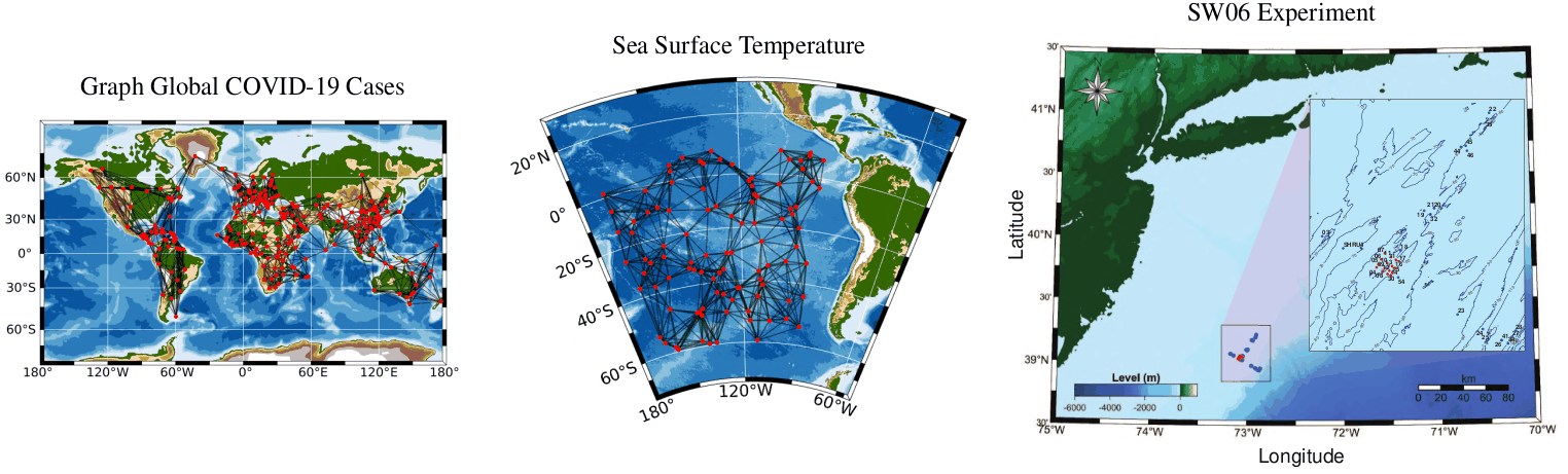
So far the data has been static: one signal on one graph. This note adds time. A sensor network reports a temperature every ten minutes, a road network reports a speed every five, a global monitoring system reports a case count every day. The graph describes where; the time series describes when; and the two are not independent.
Two problems organize the note. Reconstruction: values are missing, and we want them back. Forecasting: we have the past, and we want the future. Both are solved twice — once by writing an optimization problem, once by training a network — and comparing the two is the point of the lecture. Along the way we need one tool we have so far avoided: the spectral view of a graph.
1 Learning objectives
After studying this note, you should be able to:
- define a time-varying graph signal and the temporal difference operator;
- define the graph Fourier transform and interpret its coefficients as graph frequencies;
- express a graph filter in the spectral domain and state the cost of doing so;
- write the ChebConv recursion and explain why it avoids the eigendecomposition;
- formulate reconstruction as a smoothness-regularized optimization problem and solve it by gradient descent;
- formulate forecasting as auto-regressive modeling on a graph, and extend it to multiple horizons.
2 Time-varying graph signals
Notation in this lecture
\(M\) here is the number of time samples, not the edge count as in Lecture 1 or the mini-batch size as in Lecture 3; edge count is written \(|\mathcal{E}|\). \(N\) is the number of nodes, so \(\mathbf{X}\in\mathbb{R}^{N\times M}\) is nodes-by-time. Graphs are undirected with nonnegative weights, and \(\mathbf{L}\) is the symmetric Laplacian unless stated otherwise. \(k\) counts polynomial terms, whose degree is \(k-1\).
Definition 1 — Time-varying graph signal
Let \(\mathcal{G}\) have \(N\) nodes. A time-varying graph signal is
\[ \mathbf{X}=[\mathbf{x}_1,\mathbf{x}_2,\ldots,\mathbf{x}_M]\in\mathbb{R}^{N\times M}, \]
where \(\mathbf{x}_s\in\mathbb{R}^{N}\) is a graph signal on \(\mathcal{G}\) at time \(s\). Row \(i\) is the time series observed at node \(i\); column \(s\) is a snapshot of the whole network.
Definition 2 — Temporal difference operator
\(\mathbf{D}_{h}\in\mathbb{R}^{M\times(M-1)}\) is the first-difference operator,
\[ \mathbf{D}_h= \begin{bmatrix} -1 & & &\\ 1 & -1 & &\\ & 1 & \ddots &\\ & & \ddots & -1\\ & & & 1 \end{bmatrix}, \qquad \mathbf{X}\mathbf{D}_h=[\mathbf{x}_2-\mathbf{x}_1,\ \mathbf{x}_3-\mathbf{x}_2,\ \ldots,\ \mathbf{x}_M-\mathbf{x}_{M-1}]. \]
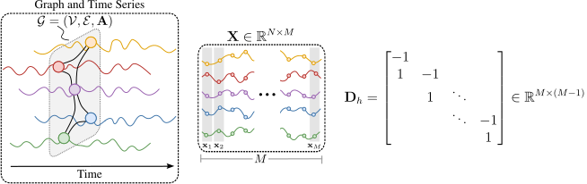
\(\mathbf{X}\mathbf{D}_h\) looks like a technicality. It is not: it is the single modeling assumption that makes reconstruction work, and Section 4 measures why.
2.1 The two problems
Check 1 — Which is which?
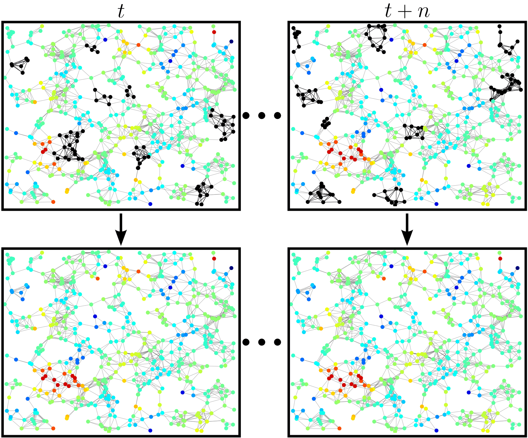
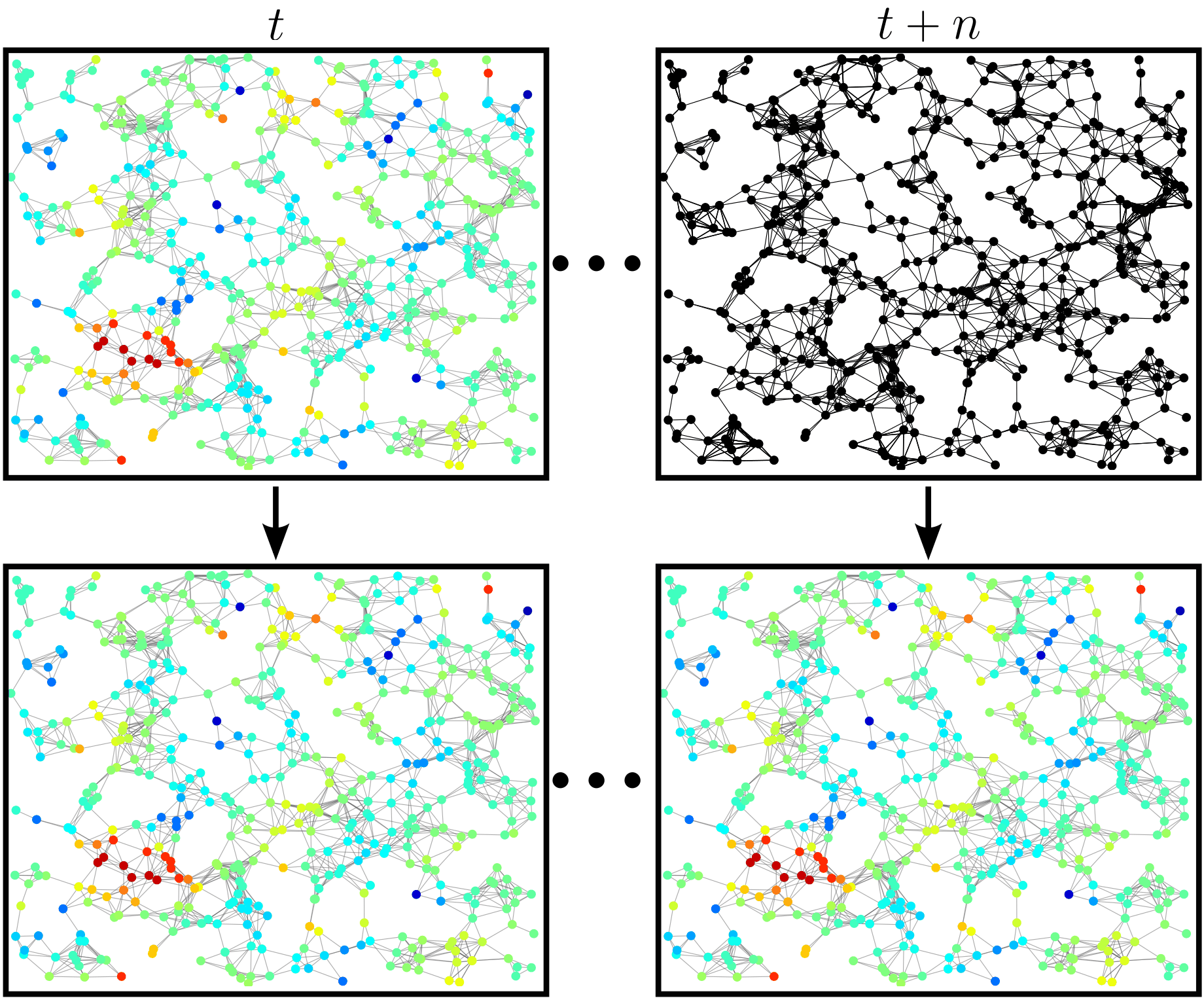
Both problems produce missing values, and it is worth being precise about the difference. In reconstruction the missing entries are interior: we know values before and after them, at the same node and at neighboring nodes, and we interpolate. In forecasting the missing entries are at the boundary: everything we know lies in the past, and we extrapolate.
Interpolation can lean on smoothness in both directions. Extrapolation cannot, which is why the two get different machinery.
3 Spectral GNNs
Lecture 2 defined a graph filter as a polynomial in the shift operator, \(\mathbf{z}=\sum_{k}h_k\mathbf{S}^{k}\mathbf{x}\), and worked entirely in the vertex domain. There is a second description, and for spatiotemporal problems it earns its keep: in practice spectral GNNs often outperform plain message passing on these tasks.
3.1 From Fourier to graph Fourier
The classical Fourier transform decomposes a signal into sinusoids of increasing frequency, and the inverse transform reassembles it.
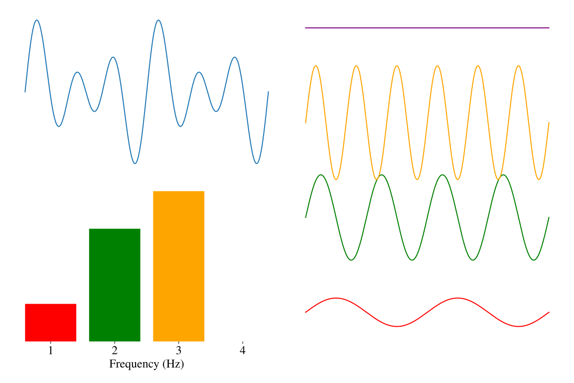
The graph Fourier transform is the same idea with the sinusoids replaced by the eigenvectors of the shift operator.
Definition 3 — Graph Fourier transform
Throughout this section, take \(\mathcal{G}\) undirected with nonnegative weights and \(\mathbf{S}\) its symmetric Laplacian \(\mathbf{L}\) (or \(\hat{\mathbf{L}}\)). Symmetry is what guarantees a real spectrum and a real orthonormal eigenbasis; a general diagonalizable shift operator can have complex eigenvalues and eigenvectors, and choosing an undirected graph does not by itself force every shift operator on it to be symmetric.
With that fixed, write \(\mathbf{S}=\mathbf{U}\boldsymbol{\Lambda}\mathbf{U}^{-1}\). The eigenvectors \(\mathbf{u}_i\) form a basis of \(\mathbb{R}^{N}\), so any graph signal can be written as
\[ \mathbf{x}=\mathbf{U}\hat{\mathbf{x}}, \qquad \hat{\mathbf{x}}=\mathbf{U}^{-1}\mathbf{x}, \]
where \(\hat{\mathbf{x}}\) is the graph Fourier transform (GFT) of \(\mathbf{x}\).
For an undirected graph \(\mathbf{S}\) is symmetric, so \(\mathbf{U}\) is orthogonal, \(\mathbf{U}^{\top}\mathbf{U}=\mathbf{U}\mathbf{U}^{\top}=\mathbf{I}\), and the pair simplifies to \(\mathbf{x}=\mathbf{U}\hat{\mathbf{x}}\), \(\hat{\mathbf{x}}=\mathbf{U}^{\top}\mathbf{x}\).
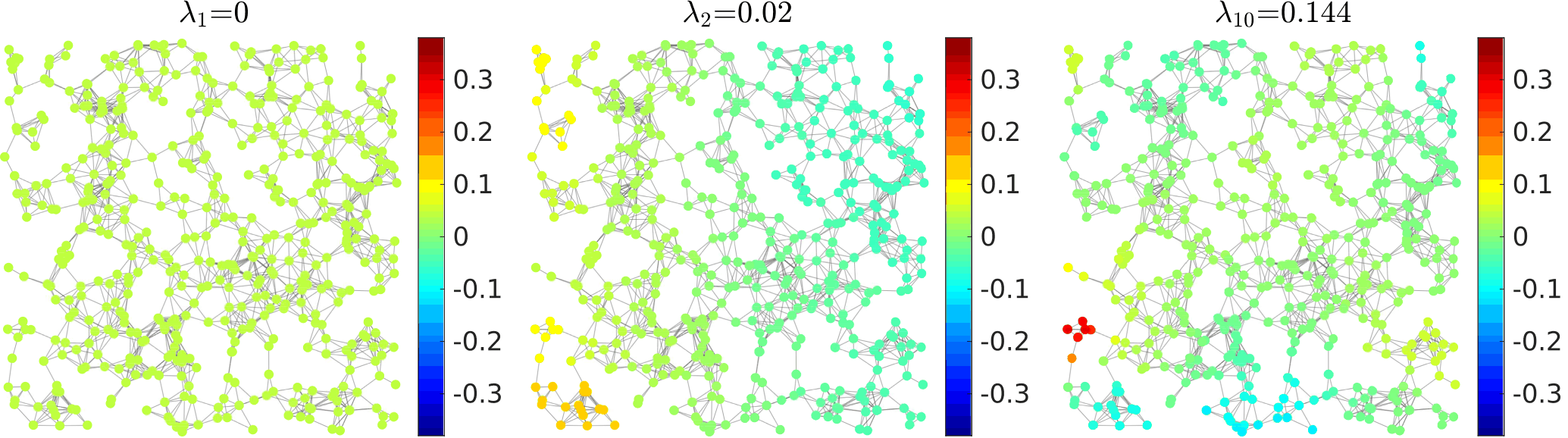
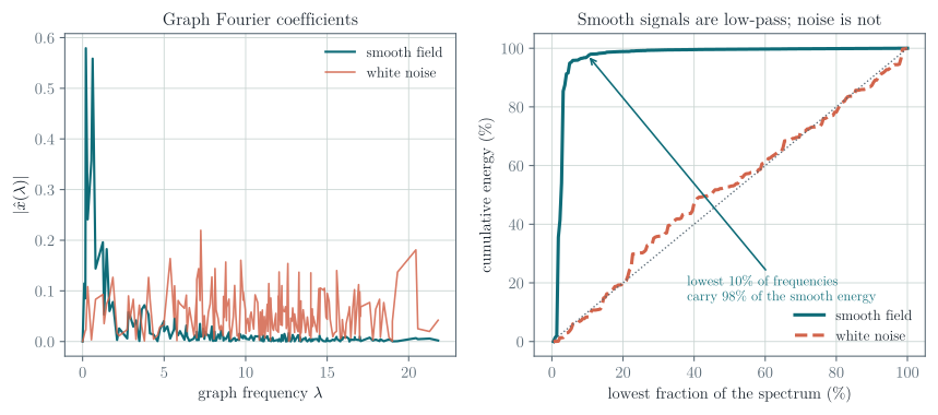
Because \(\mathbf{U}\) is orthogonal, \(\hat{x}(i)=\langle\mathbf{u}_i,\mathbf{x}\rangle\): the \(i\)-th GFT coefficient measures how similar \(\mathbf{x}\) is to the \(i\)-th eigenvector. A signal whose energy sits in the first few coefficients is smooth — it barely changes across edges. A signal spread across the spectrum is rough.
3.2 Filters in the frequency domain
Definition 4 — Graph filters in the spectral domain
Any graph filter defined as a polynomial in \(\mathbf{S}\) can be written
\[ \mathbf{H}=h(\mathbf{S})=\sum_{i=0}^{k}h_i\mathbf{S}^{i}=\mathbf{U}\,h(\boldsymbol{\Lambda})\,\mathbf{U}^{-1}, \]
where \(h(\boldsymbol{\Lambda})\) is diagonal with entries \(h(\lambda_j)=\sum_{i=0}^{k}h_i\lambda_j^{i}\) (Ortega 2022).
The proof is one line: \(\mathbf{S}^{i}=\mathbf{U}\boldsymbol{\Lambda}^{i}\mathbf{U}^{-1}\) because the inner \(\mathbf{U}^{-1}\mathbf{U}\) factors cancel; summing over \(i\) gives the result.
So filtering can be done in three steps: transform, multiply, transform back.
\[ \hat{\mathbf{x}}=\mathbf{U}^{-1}\mathbf{x}, \qquad \hat{\mathbf{y}}=h(\boldsymbol{\Lambda})\hat{\mathbf{x}}, \qquad \mathbf{y}=\mathbf{U}\hat{\mathbf{y}}. \]
This is appealing: no matrix powers, no sequential recursion, and complete freedom over the response \(h(\lambda)\) — it need not be a low-pass filter, which is exactly the limitation Lecture 2 identified in GCN.
Check 2 — The trade-off between spectral and spatial
The catch is \(\mathbf{U}\). Obtaining it requires an eigendecomposition, costing \(O(N^{3})\), and \(\mathbf{U}\) is dense even when \(\mathbf{S}\) is sparse. Compare with the vertex domain, where a \(K\)-tap filter costs \(O(K|\mathcal{E}|)\) and touches only \(K\)-hop neighborhoods.
So the spectral view is a modeling tool for small and medium graphs, and an analysis tool for large ones. Transfer is also limited, though the reason is specific: \(\mathbf{U}\) and the eigenvalue indices belong to one graph, so a model whose parameters are attached to them — one free coefficient per index, as in the earliest spectral GNNs — cannot move to another graph. A model that learns a function of \(\lambda\), such as a polynomial, has no such problem: ChebConv’s coefficients transfer perfectly well. Non-inductivity is a property of the parameterization, not of the spectral viewpoint.
3.3 Chebyshev graph convolutions
The way to keep the spectral expressiveness without paying \(O(N^{3})\) is to approximate the response \(h(\lambda)\) by a polynomial — which returns us to the vertex domain, where polynomials in \(\mathbf{S}\) are sparse products. ChebConv (Defferrard et al. 2016) does this with the Chebyshev basis, and it is the direct predecessor of GCN.
Definition 5 — ChebConv layer
\[ \mathbf{H}^{(\ell+1)}=\sum_{i=1}^{k}\mathbf{Z}_i\mathbf{W}_i, \]
with
\[ \mathbf{Z}_1=\mathbf{H}^{(\ell)}, \qquad \mathbf{Z}_2=\tilde{\mathbf{L}}\mathbf{H}^{(\ell)}, \qquad \mathbf{Z}_i=2\tilde{\mathbf{L}}\mathbf{Z}_{i-1}-\mathbf{Z}_{i-2}, \]
and the rescaled Laplacian \(\tilde{\mathbf{L}}=\dfrac{2\mathbf{L}}{\lambda_N}-\mathbf{I}\).
Two details explain the design. The rescaling maps the spectrum of \(\mathbf{L}\) from \([0,\lambda_N]\) onto \([-1,1]\), which is where the Chebyshev polynomials are defined and where they are numerically well behaved. And the three-term recursion \(T_m(x)=2xT_{m-1}(x)-T_{m-2}(x)\) is exactly the recursion satisfied by the \(\mathbf{Z}_i\).
Mind the offset, because it is easy to be one out. With \(\mathbf{Z}_1=\mathbf{H}^{(\ell)}\) the indexing is
\[ \mathbf{Z}_i=T_{i-1}(\tilde{\mathbf{L}})\,\mathbf{H}^{(\ell)}, \]
so a sum over \(i=1,\dots,k\) has \(k\) terms but degree \(k-1\), and costs \(k-1\) sparse products. Throughout this note \(k\) counts terms; when a paper says “order \(K\)” it usually means the degree, one less.
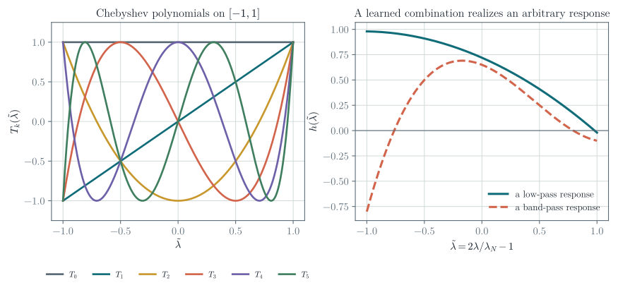
Swapping the polynomial family gives other models: Gegenbauer polynomials yield GegenConv (Castro-Correa et al. 2024), Jacobi polynomials yield JacobiConv (Wang and Zhang 2022).
Check 3 — Spectral GNNs in one paragraph
The GFT diagonalizes graph filters, turning convolution into pointwise multiplication by \(h(\lambda)\) and making “graph frequency” precise. Working on the spectrum directly costs an \(O(N^{3})\) eigendecomposition. ChebConv recovers an arbitrary polynomial response using only sparse products, through the Chebyshev recursion — and GCN is the two-term case with tied coefficients, i.e. degree one.
4 Reconstruction of time-varying graph signals
Definition 6 — Reconstruction problem
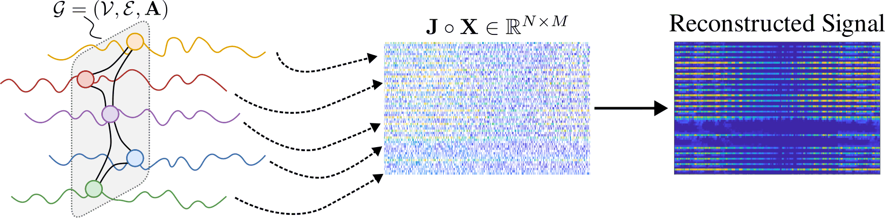
Given \(\mathcal{G}\) and a time-varying signal \(\mathbf{X}\in\mathbb{R}^{N\times M}\) in which the entries indexed by a known set \(\mathcal{S}=\{(i,j)\}\) are missing, and writing \(\mathcal{T}=(\mathcal{V}\times\mathcal{M})\setminus\mathcal{S}\) for the observed entries, recover the values on \(\mathcal{S}\).
That \(\mathcal{S}\) is known matters. We are not detecting outliers; we know exactly which sensors failed and when.
4.1 Measuring smoothness on a graph
Definition 7 — Laplacian quadratic form
\[ \Delta_{\mathbf{L}}(\mathbf{x})=\mathbf{x}^{\top}\mathbf{L}\mathbf{x}=\sum_{i\sim j}a_{ij}(x_i-x_j)^{2}, \]
summing over edges. Each edge contributes in proportion to its weight \(a_{ij}\) and to the squared difference of the signal at its endpoints.
Worked example — Computing \(\mathbf{x}^{\top}\mathbf{L}\mathbf{x}\)
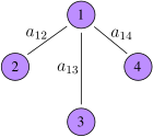
For Figure 8 the only edges are \((1,2)\), \((1,3)\) and \((1,4)\), so
\[ \mathbf{x}^{\top}\mathbf{L}\mathbf{x} =a_{12}(x_1-x_2)^{2}+a_{13}(x_1-x_3)^{2}+a_{14}(x_1-x_4)^{2}. \]
Note what is absent: no direct term in \((x_3-x_4)\). Variation is measured along edges, not between arbitrary pairs. That does not make nodes 3 and 4 free of one another — both are tied to the centre, so pushing them apart still costs through \(x_1\). What it means is that the penalty is a sum over edges, so a difference between two non-adjacent nodes is only ever penalized indirectly, through the paths joining them.
Minimum. Take \(x_1=x_2=x_3=x_4=1\). Every difference vanishes, so \(\mathbf{x}^{\top}\mathbf{L}\mathbf{x}=0\). Since \(a_{ij}\geq0\) makes every term nonnegative, this is the global minimum — and it is the constant eigenvector \(\mathbf{u}_1\) with \(\lambda_1=0\) from Figure 5.
Maximum — but only under a constraint. There is no unconstrained maximum: replacing \(\mathbf{x}\) by \(c\mathbf{x}\) multiplies the form by \(c^{2}\), so it grows without bound. The question has to be posed on a bounded set, and the answer depends which one:
- Under \(\Vert\mathbf{x}\Vert_2=1\), the maximum is \(\lambda_{\max}(\mathbf{L})\), attained at the top eigenvector. This is the Rayleigh-quotient statement and the one to remember.
- Under \(x_i\in[-1,1]\), maximizing the sign changes across edges works: \(x_1=1\), \(x_2=x_3=x_4=-1\) makes every difference \(2\), giving
\[ \mathbf{x}^{\top}\mathbf{L}\mathbf{x}=4(a_{12}+a_{13}+a_{14}). \]
4.2 From static to time-varying smoothness
The obvious extension sums the quadratic form over time:
\[ E(\mathbf{X})=\sum_{s=1}^{M}\mathbf{x}_s^{\top}\mathbf{L}\mathbf{x}_s=\operatorname{tr}(\mathbf{X}^{\top}\mathbf{L}\mathbf{X}). \]
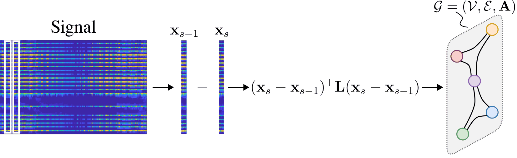
Qiu et al. (Qiu et al. 2017) observed that on real data this is the wrong quantity. What is smooth on the graph is not the signal but its temporal difference:
\[ E(\mathbf{X}\mathbf{D}_h)=\sum_{s=2}^{M}(\mathbf{x}_s-\mathbf{x}_{s-1})^{\top}\mathbf{L}(\mathbf{x}_s-\mathbf{x}_{s-1}). \]
The intuition is physical. A temperature field can have large spatial gradients — a valley is genuinely colder than a ridge — so \(\mathbf{x}_s\) need not be smooth. But when the sampling rate is high, how much things changed since the last reading is small and varies gently across the network, because neighboring sensors experience the same weather.
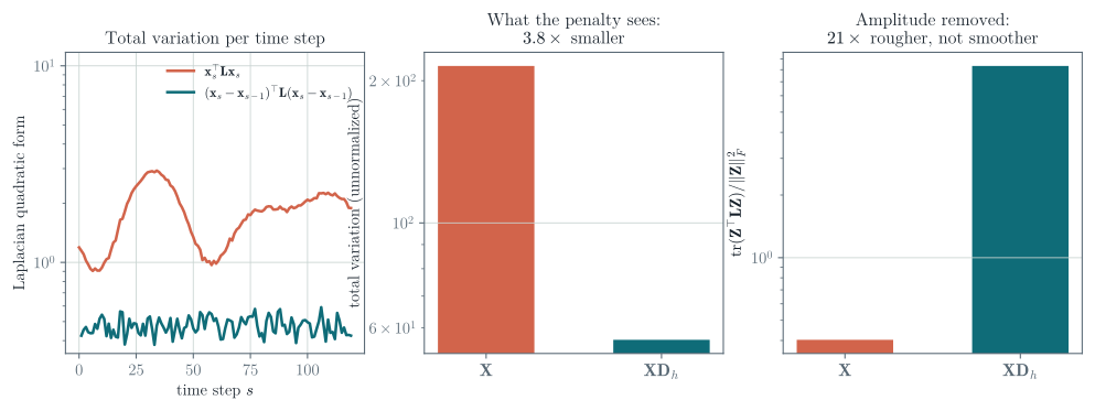
Check 4 — “Smoother” has two meanings, and only one of them holds here
This is worth slowing down for, because it is the kind of claim that is easy to assert and easy to get wrong.
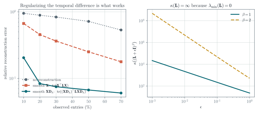
The temporal difference has \(3.8\times\) less total variation than the signal. But it also has \(78\times\) less energy: differencing consecutive snapshots of a slowly evolving field produces something small. Divide the variation by the energy and the difference comes out \(21\times\) rougher, not smoother. So the gap in the middle panel is overwhelmingly a statement about amplitude, not about relative frequency content.
Does that break the method? No — because the regularizer penalizes the unnormalized quantity. A prior works by placing the true signal near the minimizer of the penalty, and \(\mathbf{X}\mathbf{D}_h\) genuinely lands closer than \(\mathbf{X}\) does. The reconstruction experiment below confirms this directly, and that is the evidence that counts.
But state the claim carefully. “The temporal difference is smoother on the graph” is not what this experiment shows, and on this synthetic field it is false in the normalized sense — differencing is a high-pass operation in time, and here it amplifies the faster-varying modes regardless of how smooth they are in space. For the normalized claim to hold you would need the fast-changing components to also be the spatially smooth ones, which is a real physical assumption about the data, not a property of the operator \(\mathbf{D}_h\).
4.3 The optimization problem
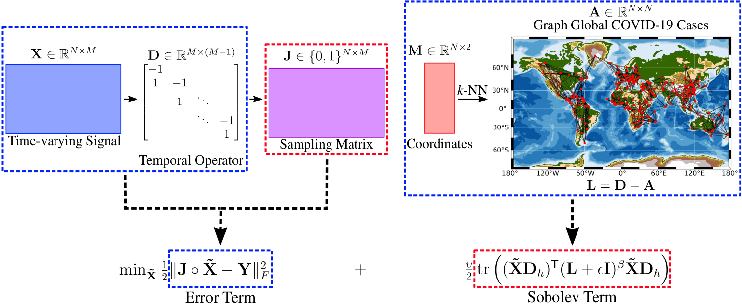
We need an error term as well. Let \(\mathbf{J}\in\{0,1\}^{N\times M}\) be the sampling matrix, with \(J_{ij}=1\) when the value at node \(i\) and time \(j\) is observed, let \(\tilde{\mathbf{X}}\) be the matrix to recover, and \(\mathbf{Y}\) the observations. Then \(\|\mathbf{J}\circ\tilde{\mathbf{X}}-\mathbf{Y}\|_F^2\) penalizes disagreement on the observed entries only — the Hadamard product simply ignores everything else.
Definition 8 — Time-varying graph signal reconstruction (TGSR)
\[ \min_{\tilde{\mathbf{X}}}\ \frac{1}{2}\left\|\mathbf{J}\circ\tilde{\mathbf{X}}-\mathbf{Y}\right\|_F^{2} +\frac{\upsilon}{2}\operatorname{tr}\!\left((\tilde{\mathbf{X}}\mathbf{D}_h)^{\top}\mathbf{L}\,\tilde{\mathbf{X}}\mathbf{D}_h\right). \tag{1}\]
4.4 Solving it
Equation 1 is a convex quadratic, so its stationary condition is a linear system. Solving it directly would mean handling an \(MN\times MN\) operator: for \(N=1000\) sensors over \(M=500\) time steps, \(500\,000\times500\,000\). Not a good idea.
Check 5 — Convex does not mean uniquely solvable
Being convex gives a global minimum; it does not give a unique one. Vectorizing, the Hessian is
\[ \mathbf{H}=\operatorname{diag}(\operatorname{vec}\mathbf{J})+\upsilon\,(\mathbf{D}_h\mathbf{D}_h^{\top}\otimes\mathbf{L}), \]
and the solution is unique exactly when \(\mathbf{H}\) is positive definite. Both terms are only positive semi-definite, so uniqueness depends on their null spaces intersecting trivially.
Here is the failure case to keep in mind. \(\mathbf{D}_h\mathbf{D}_h^{\top}\) annihilates signals constant in time, and \(\mathbf{L}\) annihilates signals constant over nodes. So if some sensor \(i\) is unobserved at every time step, adding any constant offset to that sensor’s whole series changes neither the data term (it observes nothing there) nor the temporal-difference penalty (a constant offset has zero difference). That sensor’s level is unidentifiable, and no amount of convexity recovers it.
Replacing \(\mathbf{L}\) by a positive definite \((\mathbf{L}+\epsilon\mathbf{I})^{\beta}\) fixes the node direction but not this one — the null space of \(\mathbf{D}_h\mathbf{D}_h^{\top}\) survives. Reconstruction needs a sampling condition: every sensor observed at least once, and enough coverage for the smoothness prior to bridge the gaps.
Use gradient descent instead. Writing \(f_u(\tilde{\mathbf{X}})\) for the objective,
\[ \nabla_{\tilde{\mathbf{X}}}f_u(\tilde{\mathbf{X}}) =\mathbf{J}\circ\tilde{\mathbf{X}}-\mathbf{Y} +\upsilon\,\mathbf{L}\tilde{\mathbf{X}}\mathbf{D}_h\mathbf{D}_h^{\top}, \]
a formula built entirely from sparse products. The original paper uses conjugate gradient.
4.5 Sobolev smoothness
Giraldo et al. (Giraldo et al. 2022) observed that Equation 1 is ill-posed in a specific sense, and that this slows convergence.
Check 6 — Why \(\mathbf{L}\) conditions the problem badly
The condition number of a square matrix,
\[ \kappa(\mathbf{L})=\frac{|\lambda_{\max}(\mathbf{L})|}{|\lambda_{\min}(\mathbf{L})|}, \]
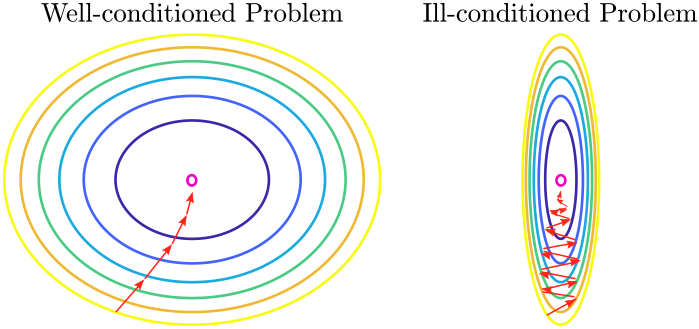
measures how well-behaved its inversion is, and small condition numbers are associated with fast convergence of gradient methods. For a graph Laplacian \(\lambda_{\min}(\mathbf{L})=0\) always — the constant eigenvector — so
\[ \kappa(\mathbf{L})=\infty . \]
The regularizer supplies no curvature at all along the constant direction.
The fix is to regularize the regularizer:
\[ \min_{\tilde{\mathbf{X}}}\ \frac{1}{2}\left\|\mathbf{J}\circ\tilde{\mathbf{X}}-\mathbf{Y}\right\|_F^{2} +\frac{\upsilon}{2}\operatorname{tr}\!\left((\tilde{\mathbf{X}}\mathbf{D}_h)^{\top}(\mathbf{L}+\epsilon\mathbf{I})^{\beta}\,\tilde{\mathbf{X}}\mathbf{D}_h\right), \tag{2}\]
adding a positive definite \(\epsilon\mathbf{I}\) so that every eigenvalue is bounded away from zero. This is called Sobolev smoothness, after its relationship to the Sobolev norm for static graph signals. The right panel of Figure 13 plots \(\kappa\big((\mathbf{L}+\epsilon\mathbf{I})^{\beta}\big)\) against \(\epsilon\): finite everywhere, and tunable through \(\epsilon\) and \(\beta\).
The algorithm changes in exactly one place, the gradient:
\[ \nabla_{\tilde{\mathbf{X}}}f_u(\tilde{\mathbf{X}}) =\mathbf{J}\circ\tilde{\mathbf{X}}-\mathbf{Y} +\upsilon\,(\mathbf{L}+\epsilon\mathbf{I})^{\beta}\tilde{\mathbf{X}}\mathbf{D}_h\mathbf{D}_h^{\top}. \]
Check 7 — What is and is not shown here
Figure 13 establishes two things directly: the temporal-difference prior is dramatically better than the static one, and \(\kappa(\mathbf{L}+\epsilon\mathbf{I})^{\beta}\) is finite while \(\kappa(\mathbf{L})\) is not.
It does not show a convergence speed-up from the Sobolev term. On this small synthetic problem the data term already supplies curvature in the directions that matter, so the two objectives descend at nearly the same rate. The empirical advantage reported in (Giraldo et al. 2022) is measured on real datasets, and you should read the paper rather than take it from a 220-node simulation. Reproducing it — or failing to — is Exercise 6.
4.6 Reconstruction with a neural network
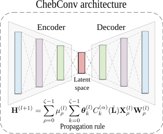
The same problem can be solved by learning. Feed the Laplacian and the incomplete signal to a GNN with an autoencoder shape, and train it with a loss that is the previous objective in disguise.
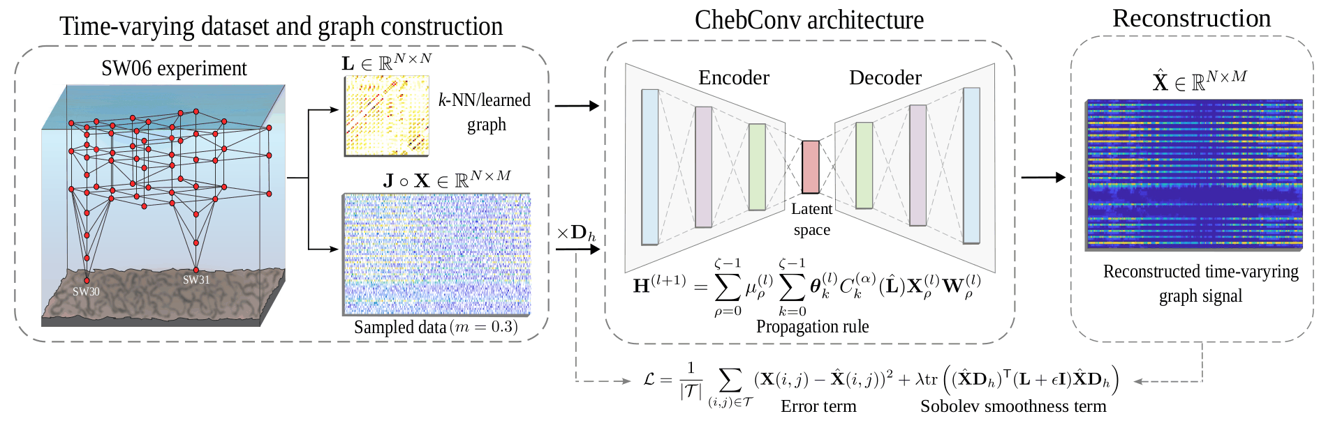
Each layer is a cascade of Chebyshev convolutions of increasing order \(\rho=0,\dots,\zeta-1\), combined linearly.
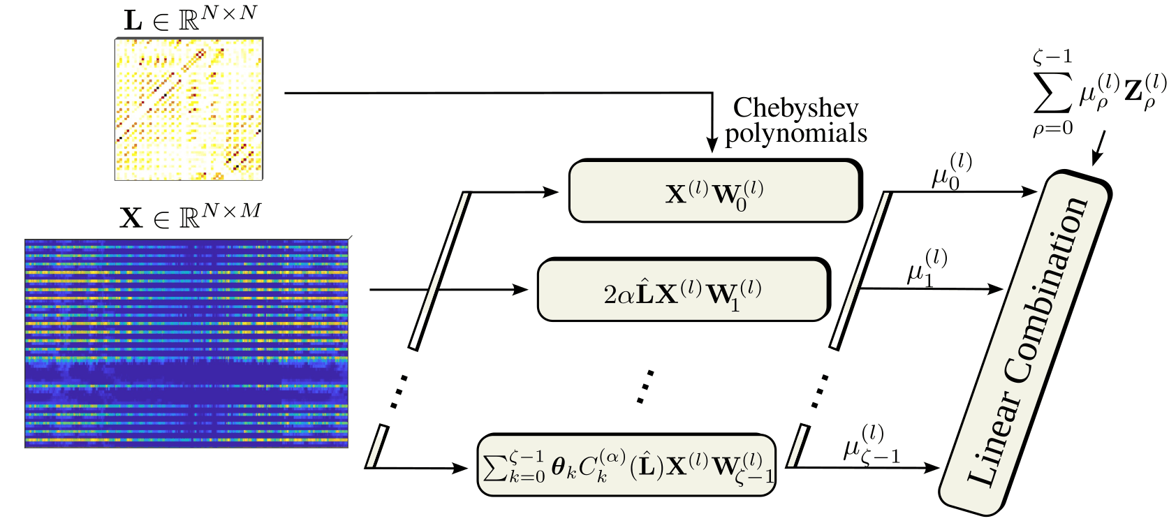
\[ \mathbf{X}^{(\ell+1)}=\sum_{\rho=0}^{\zeta-1}\mu_{\rho}^{(\ell)}\mathbf{Z}_{\rho}^{(\ell)}\in\mathbb{R}^{N\times F_\ell}, \]
where \(\mathbf{Z}_{\rho}^{(\ell)}\in\mathbb{R}^{N\times F_\ell}\) is branch \(\rho\)’s output and the \(\mu_{\rho}^{(\ell)}\) are trainable. The number of branches \(\zeta\) is a hyperparameter.
Worked example — Shapes through the autoencoder
The input is the whole time-varying signal, \(\mathbf{X}^{(0)}\in\mathbb{R}^{N\times M}\): each node’s feature vector is its time series, so the feature dimension is \(M\).
The first layer’s weights are \(\mathbf{W}_{\rho}^{(0)}\in\mathbb{R}^{M\times F_0}\) for every branch \(\rho\), with \(F_0<M\) — the encoder compresses. Widths keep shrinking to the latent layer, then grow back, and the last layer uses \(\mathbf{W}_{\rho}^{(\ell)}\in\mathbb{R}^{F_\ell\times M}\) so the output is again \(N\times M\).
These networks are shallow in practice. The reason is Lecture 2’s: over-smoothing. Depth here buys receptive field on the graph, and pays for it in discriminative power.
The loss is the optimization objective, rewritten for training:
\[ \mathcal{L}=\frac{1}{|\mathcal{T}|}\sum_{(i,j)\in\mathcal{T}}\left(X_{ij}-\tilde{X}_{ij}\right)^{2} +\lambda\operatorname{tr}\!\left((\tilde{\mathbf{X}}\mathbf{D}_h)^{\top}(\mathbf{L}+\epsilon\mathbf{I})\,\tilde{\mathbf{X}}\mathbf{D}_h\right). \]
An MSE term on the observed entries plus the Sobolev term from Equation 2. Train it with Adam or SGD.
Check 8 — Optimization or network?
They solve the same problem with the same prior, and the difference is where the effort goes.
The optimization approach has no training data, no training phase, and few hyperparameters (\(\upsilon\), \(\epsilon\), \(\beta\)); it needs a bespoke solver, and it starts from scratch on every new signal.
The network approach reuses a standard optimizer and can amortize the cost across signals; but hyperparameter tuning is harder, and it needs data to train on.
Be precise about that amortization, because it does not come for free from using a network. Reuse across signals requires a training protocol in which the model sees a collection of signals — a set of incomplete matrices with known held-out entries — and is evaluated on signals it did not train on. If instead you fit the network to one incomplete matrix and read off its reconstruction, you have used a neural network as an optimizer for a single instance, and you have amortized nothing. Both setups appear in the literature; they answer different questions. You also have to specify how missing entries enter the input — a fill value, and whether the mask \(\mathbf{J}\) is itself given to the network as a channel.
5 Forecasting of time-varying graph signals
Definition 9 — Forecasting problem
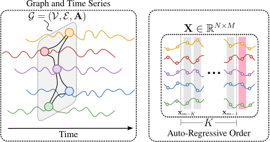
Given \(\mathcal{G}\), a time-varying graph signal \(\mathbf{X}\in\mathbb{R}^{N\times M}\), and a temporal window
\[ \mathbf{X}_K=[\mathbf{x}_{m-K},\ldots,\mathbf{x}_{m-1}]\in\mathbb{R}^{N\times K}, \qquad K<M, \]
predict \(\mathbf{x}_m\). \(K\) is the auto-regressive order.
5.1 Auto-regressive modeling
The classical AR(\(K\)) model for a scalar time series is
\[ x_m=\sum_{i=1}^{K}\phi_i x_{m-i}+\epsilon_m, \]
a weighted sum of the last \(K\) lags plus white noise. The order \(K\) sets how much history is retained, the coefficients \(\phi_i\) weight it — typically decaying with distance in time — and \(\epsilon_m\) absorbs whatever the model cannot explain.
On a graph, the scalar coefficients become matrices:
\[ \mathbf{x}_m=\sum_{i=1}^{K}\boldsymbol{\Phi}_i\mathbf{x}_{m-i}+\boldsymbol{\epsilon}_m, \qquad \boldsymbol{\Phi}_i\in\mathbb{R}^{N\times N}. \]
Leaving \(\boldsymbol{\Phi}_i\) arbitrary would be hopeless — \(KN^{2}\) parameters, and no locality. But we know from Lecture 2 what a well-behaved \(N\times N\) operator on a graph looks like: a graph filter. Take \(\boldsymbol{\Phi}_i=\sum_{j=0}^{p}h_{j,i}\mathbf{S}^{j}\) and the model becomes
\[ \mathbf{x}_m=\sum_{i=1}^{K}\sum_{j=0}^{p}h_{j,i}\mathbf{S}^{j}\mathbf{x}_{m-i}+\boldsymbol{\epsilon}_m, \tag{3}\]
with \((p+1)K\) parameters regardless of \(N\). Reading it off: the value at a node at time \(m\) depends on its own past \(K\) values and on the past values of its \(p\)-hop neighborhood. Setting \(p=1\) gives the simplest useful case, \(\mathbf{x}_m=\sum_i(h_{0,i}\mathbf{I}+h_{1,i}\mathbf{S})\mathbf{x}_{m-i}+\boldsymbol{\epsilon}_m\) — each node’s own history plus its immediate neighbors’.
Check 9 — Two axes, not one
An ordinary time series has one axis of dependence: the past. A spatiotemporal graph signal has two, and Equation 3 has one index for each — \(i\) runs over time lags and \(j\) over graph hops. Traffic at an intersection depends on that intersection an hour ago and on the upstream intersections a few minutes ago.
5.2 Forecasting with GNNs
Add nonlinearities to Equation 3 and it becomes a network:
\[ \tilde{\mathbf{x}}_m=\sum_{i=1}^{K}\alpha_i\,\sigma\!\left(\sum_{j=0}^{p}h_{j,i}\mathbf{S}^{j}\mathbf{x}_{m-i}\right), \tag{4}\]
where each lag is filtered on the graph, passed through \(\sigma\), and the \(K\) results are combined with learnable weights \(\alpha_i\).
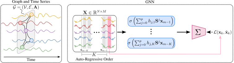
The loss is mean squared error over the nodes,
\[ \mathcal{L}_{\mathrm{MSE}}(\mathbf{x}_m,\tilde{\mathbf{x}}_m) =\frac{1}{N}\sum_{i=1}^{N}\left(x_m(i)-\tilde{x}_m(i)\right)^{2}, \]
and training is ordinary SGD or Adam.
5.3 Multiple horizons
Predicting \(H\) steps ahead rather than one admits two designs.
MLP head. Produce all \(H\) horizons in one forward pass by projecting a shared hidden representation. Let the graph layers produce \(\mathbf{Z}_m\in\mathbb{R}^{N\times F}\), with \(F\) hidden channels per node, and read out with \(\mathbf{W}_h\in\mathbb{R}^{F\times H}\):
\[ \tilde{\mathbf{X}}_m=\sigma\!\left(\mathbf{Z}_m\mathbf{W}_h\right)\in\mathbb{R}^{N\times H}, \]
with MSE taken between \(\tilde{\mathbf{X}}_m\) and \(\mathbf{X}_m\).
The width \(F\) matters. If the hidden representation is a single value per node — \(\mathbf{z}_m\in\mathbb{R}^{N\times1}\) and \(\mathbf{w}_h\in\mathbb{R}^{1\times H}\) — then the preactivation \(\mathbf{z}_m\mathbf{w}_h\) has rank one: every node’s forecast is the same \(H\)-step profile scaled by one number. That is a severe restriction, not a general head, and it is worth recognizing when you see it.
Recursive. Feed the model’s own prediction back in. Writing \(\texttt{GNN}_{\mathcal{G},\boldsymbol{\theta}}(\cdot)\) for Equation 4,
\[ \tilde{\mathbf{x}}_m=\texttt{GNN}_{\mathcal{G},\boldsymbol{\theta}}(\mathbf{x}_{m-1},\ldots,\mathbf{x}_{m-K}), \qquad \tilde{\mathbf{x}}_{m+1}=\texttt{GNN}_{\mathcal{G},\boldsymbol{\theta}}(\tilde{\mathbf{x}}_m,\mathbf{x}_{m-1},\ldots,\mathbf{x}_{m-K+1}), \]
and so on for \(H-1\) steps, assembling \(\tilde{\mathbf{X}}_m\in\mathbb{R}^{N\times H}\).
Check 10 — Two things to notice about the recursion
- The window shifts. Each step drops the oldest true observation and prepends the newest prediction, so the input stays \(K\) wide and grows progressively more synthetic.
- The parameters are shared. The same \(\boldsymbol{\theta}\) is used at every horizon — one model, applied \(H\) times, not \(H\) models.
Which is better is an empirical question, not a settled one. The recursive rollout shares parameters across horizons and matches the one-step training objective, but it is trained on true inputs and run on its own predictions — an exposure mismatch that compounds errors as \(H\) grows. The direct head avoids that compounding and can specialize per horizon, at the cost of more parameters and no guarantee of consistency between horizons. Recursive tends to do better at short horizons and on smooth, strongly auto-correlated signals; direct tends to do better at long horizons. Standard practice is to try both.
5.4 GraphCast
The clearest large-scale demonstration is GraphCast (Lam et al. 2023), DeepMind’s medium-range weather model.
- It forecasts up to 10 days ahead, learning from historical reanalysis data instead of integrating the equations of motion numerically.
- The atmosphere is encoded from a latitude–longitude grid onto a global multi-mesh graph built on hierarchical icosahedral meshes, processed there, then decoded back to the grid. The mesh is where the message passing happens, which avoids the pole distortion a regular grid suffers; the grid is still the input and output format.
- Message passing across mesh resolutions propagates information locally and globally in the same forward pass.
- It is auto-regressive, exactly as above: each output state is computed from previous states plus multi-resolution message passing.
- It produces a 10-day forecast in under a minute on one TPU, against roughly an hour for traditional numerical weather prediction.
GraphCast has a good deal of additional machinery. The part that matters here is that its skeleton is Equation 4.
Traffic forecasting is the other standard benchmark family: MetrLA (four months of speeds on 207 Los Angeles County highway sensors at 5-minute resolution) and PemsBay (six months at 325 Bay Area stations, also 5-minute).
6 Exercises
6.1 Exercise 1 — Reading the GFT
Take the path graph on 6 nodes. Compute \(\mathbf{L}\), its eigenvalues and eigenvectors, and verify that the eigenvector for \(\lambda_1=0\) is constant and that the number of sign changes grows with \(\lambda\).
6.2 Exercise 2 — Quadratic form
For Figure 8 with \(a_{12}=2\), \(a_{13}=1\), \(a_{14}=1\) and \(\mathbf{x}=[1,0,-1,2]^{\top}\), compute \(\mathbf{x}^{\top}\mathbf{L}\mathbf{x}\) directly from the edge sum, then again as a matrix product, and confirm they agree.
6.3 Exercise 3 — Why the difference is smoother
Let each node carry \(x_s(i)=f(i)+g(s)\): a fixed spatial pattern plus a spatially uniform temporal drift. Show that \(\mathbf{x}_s^{\top}\mathbf{L}\mathbf{x}_s\) is generally nonzero while \((\mathbf{x}_s-\mathbf{x}_{s-1})^{\top}\mathbf{L}(\mathbf{x}_s-\mathbf{x}_{s-1})=0\) exactly. Relate this to Figure 10.
6.4 Exercise 4 — The gradient
Derive \(\nabla_{\tilde{\mathbf{X}}}f_u\) for Equation 1. You will need \(\nabla_{\mathbf{Z}}\operatorname{tr}(\mathbf{Z}^{\top}\mathbf{A}\mathbf{Z})=2\mathbf{A}\mathbf{Z}\) for symmetric \(\mathbf{A}\), and the chain rule through \(\mathbf{Z}=\tilde{\mathbf{X}}\mathbf{D}_h\).
6.5 Exercise 5 — Chebyshev recursion
Verify that \(\mathbf{Z}_i=2\tilde{\mathbf{L}}\mathbf{Z}_{i-1}-\mathbf{Z}_{i-2}\) with \(\mathbf{Z}_1=\mathbf{H}^{(\ell)}\) implements \(T_{i-1}(\tilde{\mathbf{L}})\mathbf{H}^{(\ell)}\) — note the index offset. State the degree and the number of sparse products for a sum over \(i=1,\dots,k\). Then explain why \(\tilde{\mathbf{L}}=2\mathbf{L}/\lambda_N-\mathbf{I}\) rather than \(\mathbf{L}\) itself.
6.6 Exercise 6 — Does the Sobolev term speed things up?
Using scripts/figures/lecture_04_figures.py, run gradient descent on Equation 1 and on Equation 2 from the same start, and plot the error against iteration. Try to find a regime — sparser sampling, larger \(\upsilon\), larger \(\epsilon\) or \(\beta\) — in which the Sobolev version converges measurably faster. If you cannot, say what that tells you about which term controls the conditioning of this particular problem, and read (Giraldo et al. 2022) for the setting where the effect is visible.
6.7 Exercise 7 — Parameter count
For Equation 3 with \(N=10^{4}\) nodes, order \(K=12\) and \(p=3\) hops, count the parameters. Compare with an unconstrained \(\boldsymbol{\Phi}_i\in\mathbb{R}^{N\times N}\), and with an LSTM run independently at each node with hidden size 64.
6.8 Exercise 8 — Horizons
Explain why the recursive rollout compounds errors while the direct head does not. Then set up the comparison rather than assuming its outcome: name two properties of a signal that would favour the recursive strategy and two that would favour the direct one, and describe the experiment — horizons, splits, baselines — that would decide between them for a given dataset. Persistence (predict \(\mathbf{x}_{m-1}\) for every horizon) is the baseline both must beat.
7 Main takeaways
- A time-varying graph signal \(\mathbf{X}\in\mathbb{R}^{N\times M}\) carries a time series at every node; the temporal difference \(\mathbf{X}\mathbf{D}_h\) is the object most of the modeling acts on.
- The GFT diagonalizes graph filters and makes “graph frequency” precise: the eigenvalue is the frequency, and smooth signals concentrate their energy at the low end.
- Working on the spectrum directly costs an \(O(N^{3})\) eigendecomposition, and parameterizing per eigenvalue index does not transfer between graphs. ChebConv learns a function of \(\lambda\) instead, buying a polynomial response with sparse products only; GCN is its degree-one, tied-coefficient case.
- Reconstruction is an error term on the observed entries plus a smoothness regularizer, and the regularizer belongs on \(\mathbf{X}\mathbf{D}_h\) — worth several factors of accuracy here. The reason is that the temporal difference has far smaller total variation, which is what the penalty sees; it is not smoother in the energy-normalized sense, and Check 4 shows why the distinction matters.
- \(\kappa(\mathbf{L})=\infty\) because \(\lambda_{\min}(\mathbf{L})=0\). Sobolev smoothness replaces \(\mathbf{L}\) with \((\mathbf{L}+\epsilon\mathbf{I})^{\beta}\), making that factor’s conditioning finite and tunable — but it does not remove the null space of \(\mathbf{D}_h\mathbf{D}_h^{\top}\), so uniqueness still needs a sampling condition (Check 5).
- The same problem solves with a polynomial-filter autoencoder and the same loss. Optimization needs no data; the network can amortize across signals, but only under a training protocol that actually trains on a collection of them. Both are shallow, for the usual reason.
- Forecasting is auto-regressive modeling where the AR coefficients become graph filters, giving dependence on both past time steps and nearby nodes with a parameter count independent of \(N\).
- Multiple horizons come from a direct head on an \(N\times F\) hidden representation or a recursive rollout with shared parameters; which wins is an empirical question, and both must beat persistence. GraphCast is this recipe at planetary scale, encoding from and decoding to a latitude–longitude grid while processing on a multimesh.
References and provenance
This web note is adapted from the Lecture 4 slides by Jhony H. Giraldo. The graph-filter diagonalization is proved, the shapes of the autoencoder are worked through, the auto-regressive model is derived from the classical AR(\(K\)) model, and the smoothness and conditioning claims are checked numerically.
The diagrams reproduce the original course vectors. Figure 6, Figure 10, Figure 13, and Figure 7 are new and were computed with numpy and networkx; the script that produces them is scripts/figures/lecture_04_figures.py in this repository. Figure 4 is a redrawn version of the lecture’s Fourier recap.